So it is off a Touch, So What?

With billions of dollars invested and trillions at risk, how accurate should the climate data be? That question will cause many to proclaim I am a merchant of doubt. I don't make a living selling doubt but I do have a pretty good inventory. The chart above compares the gold standard surface station temperature data for the Southern Hemisphere with the state of the art satellite telemetry data for the same region. The University of Alabama, Huntsville data compiled by Dr. Roy Spencer is a bit controversial. Another group, Remote Sensing Systems (RSS) also has a satellite temperature product that is comparable. The UAH currently has a slightly higher trend over the period than the RSS group's. Doubters can make their own comparison. The trends in the above plot are 0.0107 degrees per year for the GISS surface station data and 0.0019 for the UAH data. So in one hundred years, if nothing changes, the Southern Hemisphere would be 100*0.0107=1.07 degrees warmer or 100*0.0019=0.19 degrees warmer. Now this is just the land mass temperatures for the bottom half of the planet which has more water than it does land mass. Most of us live in the Northern Hemisphere where we KNOW it is warmer.

Let's see, 100*0.0637=6.37, so if nothing changes, according to NASA GISS Northern Hemisphere land only surface temperatures it will be 6.37 degrees C warmer in 100 years. Pretty alarming huh? 100*0.092=0.92degrees C warmer in one hundred years based on the high dollar satellite data. The two sets disagree. They significantly disagree. That is not that unusual, what they are attempting to do is pretty damn hard, averaging the surface temperature of the whole planet by less than adequate means. So what's a guy to do? This guy compares something that is known to be happening to both. There are pretty good measurements of CO2 concentration from the Mauna Loa Observatory, increasing CO2 does have a radiant impact and that impact will have a relationship with temperature that is a natural log curve fit. Where on that curve is a question and that means that the magnitude of the impact is in question, but it will fit a natural log curve fairly well. You can prove that to yourself with some ink, and aquarium and your eyeballs if properly calibrated, a light meter is not. Start with clear water, add a half of drop of black ink at a time and measure the change in the light passing through the tank. The change will roughly match a natural log curve. Just for fun, use a rectangular tank and measure the light change from front to back and from side to side also. If you look up at the night sky, that is side to side, if you look up from a very high mountain top up, that is front to back. More on that later. Right now, here is my check.

The blue squiggly line in the middle of that plot is the estimate forcing due to CO2 increase since 1979 and it is compared to the global land only UAH satellite data. 100*0.0082=0.82 degrees C if nothing changes with the CO2 and 100*0.0080=.80 if nothing changes for the land temperature data. That is fairly good agreement. Note that the satellite data is all middle troposphere data. The data that should be warmer than the surface. Think about the aquarium for a second. Now assuming that nothing changes is not all that bright. Things do and will change but it is nice to have a somewhat reliable baseline to determine how much and what changed. Without getting into a graph, here is a quick check for the GISS data. The GISS data says the Southern Hemisphere is warming. The Antarctic sea ice is at record levels for the satellite era, which is about the only data we have on Antarctic sea ice. Would Antarctic sea ice be growing and at record levels if the Antarctic were warming? That Arctic sea ice is declining in summer. Is it declining in winter? There has been some decline in winter Arctic sea ice, but not a huge amount. Summer ice has either set or come close to setting a minimum record in 2007. This gives us a little logical check of GISS. Yes there has been warming in the Northern Hemisphere and it is unlikely there has been significant warming in the Southern Hemisphere. One thing is certain, there is definitely more seasonal change in the area and perhaps volume of sea ice globally since the start of the satellite era. Now a neat fun fact. Sea ice growth, drives the deep ocean currents. When salt water freezes, it losses some of the salt content so the actual ice formed is fresher than the water that formed it. That salt is lost to the unfroze water where it increases the density of that water which sinks deeper than the less dense water surrounding it. The more sea ice formed, the greater the volume of sinking, more dense, water. This water would be very close to the freezing point of fresh water, 0 C or 32 F. The deep oceans are not frozen, so the denser water settles into a thermal layer of approximately the same density beneath the surface. This sinking water must force some less dense water toward the surface. This creates a deep ocean current, falling cold dense water and rising less dense water. If the rate of sea ice production increases, the rate of the deep water cold current increases. That water is always at the same temperature as it is set by the freezing point of the water salinity. Now the harder part. With more rapid ice melt, the surface water would be fresher than normal, unless winds and currents mix the fresher melt water with the more saline ocean water. In the Antarctic, there is no indication of summer melt increase but evidence of increased winter formation, so there has been an increase in flow into the deep ocean current. In the Arctic, it really depends on which way and how strong the wind blows. So GISS gets a no go in the Antarctic and Southern Hemisphere and a grudging maybe in the Northern Hemisphere. So should we spend trillions of dollars because of a grudging maybe? I don't think so. There is still quite a bit of work to be done before we can predict climate.

What the Flux!T

hat is a busy chart comparing the Mauna Loa CO2 concentration change estimated forcing to the University of Alabama (UAH) Microwave Sounding Unit (MSU) middle tropospheric temperature data. The light blue line burried in the noise is the calculated forcing of CO2 based on the formula 5.35ln(Cf/co) were Co is 280 Parts Per Million PPM. Cf is the monthly average from the Mauna Loa observatory CO2 measurements. Since the UAH data is in anomalies, I converted the CO2 forcing estimate to Anomalies by subtracting the average of the period of the satellite data series.

Low and behold, the CO2 forcing is nearly a perfect fit of the UAH land temperature data series. Both the global and the ocean series are below the land series.

This chart is just the land data and the estimated CO2 forcing. Pretty close match. If you extend the regressions out to the year 2100, it is about 0.8 C greater than the start in 1979. Now here is a little bit of a shocker, CO2 is causing most of that warming. But why is it only a good match over land?

The average surface temperature of the Earth is often listed as 288K degrees with a outgoing energy flux of 390Wm-2. Average temperature, average flux right? The average temperature of the oceans, 70% of the global surface is about 294K degrees and the average temperature of the land area is about 273K degrees. The energy flux at 294K degrees is about 423.6Wm-2 and the flux at 273.15 is about 315.6Wm-2. .7*294+.3*273.15=287.7 and .7*423.6+.3*315.6=391.2 the temperature is a touch lower and the flux a touch higher. Small errors right?

If you add 3.7Wm-2 of forcing to a 273.13K surface it would increase to 273.9K. Add 3.7Wm-2 of forcing to a surface at 294K and it would increase the temperature to 294.6K, only 80% of the increase. If you estimate the increase in forcing based on an average of temperatures instead of an average of fluxes, you get a slightly high bias in your estimate. Then if you apply the slightly high estimate to an average of temperatures you would get a slightly low response. This is exactly what appears to have happened to the climate change projections.

This does not explain all of the discrepancies, but since the oceans appear to also have a negative water vapor feedback, it should explain a large percentage of the error.

What's a Watt?

A Watt is a unit of energy flow or power named after James Watt, the steam engine guy. There are lots of energy terms. According to Wikipedia, a Watt is defined as a Joule/second which is a measure of energy conversion or transfer. Since it is a flow thingy, you have to know the area it is flowing through and how long it is flowing. The units for the power then is in Watts per meter squared per some period of time. Since it is defined as a Joule per second, there are 60 seconds in a minute and 60 minutes in an hour, there are 3600 Joule/seconds in a Watt hour. A kilowatt hour would be 3,600,000 Joule seconds.

So should I say that there is only 0.1 Joules/second-meter squared of energy flow, that would be tiny. If that flow was through the surface of the Earth with an area of 510,000,000 kilometers squared which is 510,000,000,000,000 meters squared, it would still be small to most folks thinking. At 0.1 Wm-2, that would be 5.1 x 10^13 Joules per second or Watt-seconds. Since there are 3.6 x 10^6 Joules per kilowatt-hour, that would only be 1.42 x 10^7 Kilowatts per hour. That is about 14.2 GigaWatts per hour. Big number, but still small to most folks.

In order for those folks to consider it significant, it takes more time, say 40 years. There are 60x60x24x365.25x40 equals 1.26 x 10^9 seconds in 40 years. I have lived more that that many seconds, so from experience I can tell you that is not a very long time. Now with 1.26 x 10^9 seconds and 5.1 x 10^13 Joules per second you end up with 6.44 x 10^22 Joules. That seems like a lot of Joules. Still that is not much to some folks. Those folks think that 22 x 10^22 is a lot of Joules. Well it is a little over three times as much as the not so much 6.44 x 10^22 Joules. If you convert it to kilowatt hours, the number is even smaller. It is only like running a 14.2 gigawatt-hour power plant 24/7/365 for 40 years. Nothing right?

If the surface of the Earth was to cool from 288K to 287.8K, that is not much either. That would only be 1Wm-2 less energy radiating from the surface if the surface were a true black body. That is ten times as much as 0.1Wm-2, so that would be like running the 14.2 gigawatt-hour power plant for only four years, 24/7/365.

Well, the average surfacetemperature of the World's oceans is more than 288K degrees. They are closer to 294.25 K degrees. If their temperature dropped to 294.225, a 0.025 K degree drop, that would be like 0.1Wm-2 less energy, which must also be insignificant to most.

More AQUA StuffA

AQUA satellite data is not a particularly long set and with the gaps it does have issues. The chart above AQUA ocean surface temperature for the length of the series is adjust to anomalies showing seasonal variation. When the sun is in the southern hemisphere, the ocean warms more and it cools more in the southern winter. Nothing shocking about that. There appears to be a slight downward trend, but not much. To compare years, I averaged each year of the series produce an "average" season, short record, not much significance in that, just something to look at.

As you can see in the first four years, "average" is not something we can expect very often. Each year has significant variations. I did at a mean value line so that general warming or cooling for the whole year versus "average" can be seen. 2006, is the year before the great Arctic Ice Melt. It was warmer than previous years, but not by much.

Following the great ice melt, things keep on keeping on. The temperature variations increased likely to the ENSO, but the range of change is within +.06 and -0.1 degrees. I may make more comparisons of other channels with the "averages". What would be interesting is a comparison with cloud fraction.

Building a Better Model - Data Issues

I doesn't matter how elaborate a model you build of the atmosphere, if you can't verify it with data it won't fly. When you have so much data with so many conflicts and you are looking for extremely small changes, you may need a model just to determine which data is meaningful and which leads down a rabbit hole. So this is a first attempt to generate a little different twist on the satellite data to help isolate issues with the different data sets.

The Aqua data is short and has gaps. The data started in 2002 and is current, but the channel 4 data bit the dust and there are gaps in the other channels. The data is in degrees Kelvin for different atmospheric pressure levels. Channels adjacent to each other likely have some error due to proximity, so leap frogging one or more channels should reduce that error. This is a chart for channel 5 the 600millibar layers (approximately 4.3 kilometer altitude) and the 50 millibar layer, (approximately 50 millibar).

On the chart, the blue curve is an approximation of the flux imbalance between the two layers. By converting the temperature value of each layer into perfect black body flux values using the Stefan-Boltzmann relationship, the subtracting the channel 5 flux equivalent from the channel 10 flux equivalent. This was then modified to an anomaly by subtracting the average of the entire range from the daily values. Where there are gaps in either data set, those days are left blank and skipped in the plot. The orange curve is an approximation of the emissivity for the ch. 5 600 mb layer to the ch. 10 50 mb layer. This plot uses the right y axis scale. The calculation for the emissivity is flux equivalent of the ch 10 data divided by the flux equivalent of the ch. 5 data.

The emissivity of a perfect gray body should approach 0.5 unless my estimates are completely screwed up. Deviations from 0.5 should indicate that energy is converted into work, passing through the medium without interaction, being transported by other than radiant means, or something is wrong.

The limited data indicates that the emissivity between layers is above 0.5 and slowly approaching a value closer to 0.5 and that there is a fairly large seasonal swing in the flux difference between layers with than difference reducing with time. Warmer years have higher positive values. with the average reducing, that would indicate that at least for the short term that there will be some reduction in the average temperature of the 600mb layer. The fit of the two curves is very close since they are based on the same flux relationship. There is some interesting difference in the peak and valley correlation. At the peak, both the estimated imbalance and the emissivity plateau at the same relative locations. In the valleys, emissivity decrease reduces faster than the estimated flux imbalance. This may indicate that convective cooling is taking a larger role relative to radiant cooling at or below the tropopause. The valley difference may indicate a return to radiant control of cooling in the media between the two layers.

The change in the estimated emissivity is most interesting. Changes in the minimum local emissivity due to mixed phase clouds, primarily in the Arctic, cause considerable uncertainty in the energy budget estimates. With more complete data, (using surface to 150mb and other AQUA channels) plus a longer data series, better estimates of the impact of minimum local emissivity variation may be determined.

The data used was taken from the Discover AQUA site and transferred to a spreadsheet. There may be errors in the charts due to transcription errors or brain farts. The purpose of the chart is just to show a potential application of the AQUA data for atmospheric physics hobbyists.

This chart compares the approximate emissivities of the 600mb channel 5 to the higher channels up to channel 11 at 25 kilometers and 25 millibar. If Channel 4, the lowest troposphere level were available it would have the highest emissivity value. These are relative emissivities which could easily be called transmittance. Each higher layer transmits less of the emission from the channel 5 layer. So if channel 5 emits 300Wm-2 and channel 10 emits 100Wm-2, 100/300 would be .33 or the amount of channel 5 energy emitted by channel 10. Two thirds of the channel 5 energy may be emitted to space. Of course, all the energy from the higher layer need not originate at the channel 5 layer, portions could be due to short wave absorption in the atmosphere above channel 5. However, the channel 5 layer is moist an likely close to the maximum radiant layer. There is only a short section of the channel 4 layer, but I will dig that out for a comparison.

Agricultural Impact on Climate, Real and not so Real

More than one experimenter has been fooled by his own data. The world's energy problems were solve by a team of researchers at the University of Utah when they discover cold fusion. That was until they found out that their data had fooled them. Measuring temperature can be tricky.

With a significant percentage of the surface of the Earth altered by mankind to produce food, shelter and ease of transportation, that should have an impact on climate. After all, CO2 is supposed to only make a 1 percent change, a 10 percent change or better in land use should have and impact greater than CO2. Some scientist agree than land use is responsible for most of the warming, some disagree. They are all good scientists, why would there be any disagreement?

Because numbers lie.

Anyone that has ever attempted to garden knows the value of mulch. It looks great when you first install it, it slows down the growth of weeds so it looks better longer, it retains soil moisture so you don't have to water as often, and it regulates the soil temperature. The mulch can be black, that nifty red looking stuff, honey colored hay, various shades of brown or even some goofy custom color to match your house color. No matter what color, it still does the job.

Forests tend to prefer the natural color mulch which is darker brown to nearly black. Most farmer don't use mulch. So if farmers remove trees and brush to build farmland, the natural mulch is turned into the soil. The temperature over the farmland will be warmer than the temperature over the forest floor and not just because of the shade from the trees.

Mulch, despite the chosen color is an insulator. The air trapped in the loose mulch warms before the soil and convects heat away from the dirt. Dirt is an insulator, but not as good as mulch. More heat is absorbed by the deeper soil uncovered by mulch than that covered. That is a good thing for seed germination,but it tends to increase evaporation of water from the soil. The more heat that is absorbed, the more watering that is required. Remember, that is another reason gardeners like mulch.

So soil temperature will be higher in the day time without mulch. The soil will release more of that heat at night because mulch is a better insulator than soil. This has a real and a not so real impact on the average global temperature.

The real part is that the soil absorbs more energy which is measured as increased temperature. The unreal part, is that the flow of energy and reflection of solar energy impacts the temperature measurements more than the air that is attempted to be measured.

Great pains are taken to make sure that the housings of the surface station temperature measurements are consistently white, so that they absorb a uniform amount of direct solar energy. Then that very scientifically designed instrument is mounted on a pole. In most areas, that pole is now galvanized metal. In some areas it may be pressure treated lumber. It others it may be a neat bracket. The choice makes a difference in the measured temperature.

Take a few of the new digital weather stations with the neat white beehive vented housing. Mount one on a black metal pole, one on a natural wood pole and one on a wooden pole painted white. Would there be any difference in the temperature measured? Now set each a white sheet under each, would there be a temperature difference?

So you see, hopefully, part of the issues with direct measurement of surface temperature.

What generally defines the energy absorption of the surface is the albedo or the reflectivity of the surface. What defines the impact of the albedo is the retained energy. A black surface that does not retain energy has little impact on climate by a great deal of impact on temperature measurement. This is the issue with determining how much impact agriculture has had on climate. The albedo change says not much. The difference in retained energy says a whole bunch. So a more accurate measurement of climate change would be soil temperature below the surface. That is not on the list of priorities, so the next best measurements are sea surface temperature and ocean heat content.

The moral of this story is take all measurements with a grain of salt. Everything measured needs verification if it is to be relied upon.

Welcome Back Medieval Warm Period

There was a warm period in medieval times when the Vikings settled Greenland and even started to settle in the Americas near Newfoundland. That all changed because a group of scientists could not find evidence of the warm period globally. If it wasn't global it didn't count.

That created a bit of controversy, because all of us older folks had been taught that there was a Medieval Warm Period and a Little Ice Age. The global warming scientists thought that the MWP was not very big and that the LIA probably was not either. That would mean that we, mankind, where causing unprecedented warming of apocalyptic proportions. We, mankind, were all going to die or at least be in some way harmed or inconvenienced, if we do not change our productive ways quickly.

So what is the big deal about the MWP and the LIA?

That chart show a Siberian tree ring reconstruction of past temperature by Jacoby et al which is available on the NOAA paleo site. It is the Taymar or Taymyr Peninsular reconstruction, in orange. The blue plot is the Southern South American tree ring reconstruction by Nuekum et al, also on the NOAA paleo website. What is plotted are 31 year moving averages with the Taymyr reconstruction shifted forward by 25 years. Both reconstructions were adjusted to have a common mean value. The plot indicates that there is much more temperature or at least more tree growth variability in the northern Siberian region than in the southern part of South America.

This shows unprecedented warming in the orange but not so much in the blue. So it is clear that something happened more in the Taymyr area than happened in the SSA area. That something is likely us, mankind, doing something. That something was definitely farming and industry. So we, mankind, have probably had an impact on climate. Since the impact is greater in the North than the south, farming has an edge on the impact with CO2 released during industrialization coming in second. At least that is my interpretation,

There is one issue though, Taymyr does not start at the same time as SSA. By averaging over the entire length of both reconstructions, I have an average, but I do not know how those averages relate to actually temperature.

Unless the regional reconstructions realistically reproduce temperatures you don't. The plot above is for Cook et al 1998 Tasmania with the Nuekum et al 2010 Southern South America. Averaging these two together suppress some of the signal, but leaves most of the peaks intact. Average enough quality reconstructions in the southern hemisphere, you should end up with a fair reconstruction of sea surface temperature. So comparing these reconstructions to air temperature would depress the past, just like comparing land temperatures to sea surface temperatures would show greater variation of the land than the oceans.

So you compare tree ring reconstructions to global surface temperature average you get a distorted view of the past. Long term averages should be compared to sea surface temperature, not air temperature. It appears to make a huge difference.

UPDATE:

Just for grins, I figured I would build a hockey stick, but a high tech hockey stick, I am going to use the satellite data.

To start, I used the UAH southern hemisphere ocean data which I tried to match to the Hadley CRU version 2 SST data. My legend has a typo, it should be HADSST2. Since there is a bit of a dust up over the new version, I just used the one I had. Since I had already adjusted the averages for the Tasmania and Southern South America data, I shifted the two instrumental data sets to overlapping periods. I actually came out in the ballpark of what it should be as best I can tell.

Starting at 1400 AD I get the most dramatic hockey stick! Unlike most data splices, I used the 31 year moving averages for the proxies and the monthly for UAH and annual for HADSST2. So without including error bars, the noise of the instrument gives a rough idea of the range of temperatures now versus the smoothed proxy data.

This is the same data starting in 900 AD, that includes the MWP and the LIA. So today is probably warmer that those periods, but with the fluctuation of the instrumental data, it is hard to say how much.

This plot starts in the year 1 AD with all the same data. The Tasmania data goes back a lot more, but this is probably the highlight. So the only thing you can conclude is that the MWP and the LIA were global, but in the Southern hemisphere the change was probably not all that much. The big changes were in the Northern Hemisphere most likely. The funny part is that sea surface temperature doesn't look like it bothered changing much. The big changes around the end of WWII are probably just noise.

Don't Forget Land Use

“It turns out that land-use changes, right up to about 1950 or even 1970, were as large a player as fossil-fuel emissions were,” he says. “And even today they are not trivial.”, imagine that? Actually, those land use changes, since they are amplified by the greenhouse effect, are more than just not trivial, they are a pretty big deal. It is a lot easier to use agriculture to mitigate warming than it is to do wacky things in the air.

Speaking of wacky things in the air, the first natural compound every synthesized was urea. A common compound in urine and fertilizer. Urea contains a good deal of energy. A good bit of that energy is the hydrogen molecules and the CO party of the chain. So urea can be used to store energy and can be used in fuel cells. It can also be converted into liquid fuels. Since Urea production gets its CO and nitrogen from the air in most processes, it would be considered a sustainable or green energy component. It is normally produced with natural gas, but integrated gasification starting with coal or biomass by creating "syngas" or methane, can also be used.

Now, once the science guys verify that the Antarctic was cooling like the satellite data says, not the surface station data says, things will be moving along swimmingly. Crisis averted, bring on the next crisis.

My biggest question is how are the doom sayers going to save face? They did work extremely hard to scare the hell out of everyone. Tried to promote an idiotic one world government and all that. Will they still have jobs?

Time will tell.

Still Trying to Slay the Slayers

The Tyndall Gas Effect, Greenhouse Effect or the Atmospheric Effects,are all due to electromagnetic radiation interacting with the various elements that make up our atmosphere. As visual creatures, there pretty ones, rainbows, sundogs, aurora are all attention grabbers. The ones we cannot see, as with our own eyes, are more fun to explain. A book, Slaying the Sky Dragon, disputes the Greenhouse Effect, which is based on the Tyndall gas effect which is one of the Atmospheric effects invisible to the human eye. Humans tend to believe what they wish to believe until they "see" clear evidence to the contrary. The Slayers, have not seen the infrared light of the basic physics involved in our atmospheric effects. Mainly because the explanations or and analogies for the "Greenhouse effects" are not very well presented. Dr. Roy Spencer, has recently taken another stab at slaying the slayers.

I believe the main reason that the "greenhouse effect" is still causing controversy is the not that great understanding of the effect by the people trying to explain it. The impact of the Tyndall gas effect, AKA greenhouse effect is not just one, but a combination of effects. Describing one part while not acknowledging the rest, only increases the confusion.

One of the common mistakes is the insulation analogy. Everyone is familiar with home insulation and coolers for keeping things cool. Most everyone has a grasp that a cooler can keep beer cool can also keep food warm longer as well. It does both by reducing the rate of heat flow out of or into the cooler. Heat, a convenient form of energy, flow from greater to lesser or hot to cold. A cooler doesn't have a computer to let it know what it should do, the laws of physics, specifically, the laws of thermodynamics dictate what it does. They are laws, not guidelines.

Energy will find a way to find a lower level. The main paths for heat or thermal energy flow are conduction, convection and radiation. The rates of each flow depend on the medium of transmission because of thermal properties of that medium and the difference in energy or heat.

Conduction is the direct exchange of energy between molecules in contact. If you roast a marshmallow over a fire with a stick you will have a more pleasant experience than roasting the same marshmallow with a copper rod. Copper conducts heat much more efficiently than dried wood. If you use a green stick, you may find that your hand gets a bit warmer than if the stick is dry. Dry wood, copper and wet or green wood have different thermal properties.

The dry stick conducts the least heat of the three. The only difference between the green and dry sticks is the moisture. So water has a impact on heat transfer. The physical properties of water that cause the difference are it specific heat capacity and phase characteristics. Water though varies in volume. As a liquid, one kilogram of water occupies about one liter of space.

As ice, the water occupies more space. As a gas, water occupies even more space. How much space depends on the temperature and pressure of the space. Because of the physical properties of water, ice floats and steam rises. A huge amount of the Tyndall effect and all atmospheric effects is due to the properties of the substance water.

If you are in a desert, which has little water vapor in the air, You will be hotter in the daytime sun and colder at night than you would be on the ocean with the same amount of sunshine. That is because the air in the desert has a lower specific heat capacity than moist air on the ocean and it time time for heat to flow into or out of a volume.

With the green stick, it long to get hot at the handle than the copper rod and more time than the dry stick. The rate of heat flow varies with the physical properties of the medium, in this case the skewer for roasting a marshmallow.

The specific heat capacity of water is 1 calorie per gram degree C at 0 degrees C. That is one of the highest heat capacities of any substance. Since most table list specific heat in Joules, not calories, water as a liquid has a specific heat capacity of 4181J/kg or 4.18J/gram.

As a vapor, water has a specific heat capacity of 2.08J/kg and 2.11J/kg as ice. These values do change with temperature and pressure. Dry air has a specific heat capacity of 1J/kg at sea level and 0 C degrees. Water vapor has twice the heat capacity of dry air. Adding water vapor to dry air increases the heat capacity of the air mixture. Wikipedia has a nice list of the sensible heat capacities of substances. that is only a part of the story though.

Wikipedia also has a list of the thermal conductivity of substances. This list is a lot more complicated because different common substances has different compositions. Dry wood for example has a range of 0.04 to 0.17 Watts per meter-K, wet wood, at 12% moisture has a range of 0.09 to 0.4 W/m-k, but you can see that with about 12% moisture, wet wood conducts 4 times as much heat energy.

Water vapor, at one bar or at sea level conducts 0.04W/m-K or one tenth as much as the wet wood. Make a mental note of that.

The thermal conductivity of air 0.024, per the engineering toolbox. Adding moisture to the air increase the thermal conductivity. Then change in the thermal conductivity is a little confusing though. Any moisture changes the thermal conductivity, but there is no significant difference until the temperature of the moist air mixture is greater than 20 C degrees. As the temperature of the moist air approaches 100 C degrees, the difference is much larger. The reason for this it that that amount of water vapor that the air can hold is limited by its temperature and pressure.


Now water vapor can change the thermal conductivity as I ask you to note, but it is limited by the properties of the mixture of all atmospheric gases, temperature and pressure from making much change under normal atmospheric conditions. That limit is called the saturation vapor pressure. Air can be saturated with moisture which would be 100% relative humidity. Once it reaches saturation, it cannot hold any more moisture unless the temperature increases or the pressure decreases. Since the temperature in the atmosphere decreases with decreasing pressure, warm moist air can rise further in the atmosphere until it reaches a point of 100% relativity humidity and the water vapor begins to condense. Since water has a higher specific heat than water vapor, there must be a change in heat content and volume for there to be a phase change from vapor to liquid or vapor to solid. Since this change is not easily seen, it is call the latent or hidden heat of fusion or vaporization. Heat has to be gained by the water molecules to progress from ice to water liquid to water vapor, and heat lost to progress in the opposite direction. As a vapor, water is limited by temperature and pressure to the amount of energy it can gain or lose until it reaches saturation.

So water vapor adds to the specific heat of the air, causes a small increase in the thermal conductivity of air which is limited by temperature and pressure and the amount of water vapor the air can hold is limited by temperature, pressure and available water.

Back to the marshmallow roast. If it is a cold night, you will notice that the fire warms one side of you, the one facing the fire, and the back side stays cool or even seems to get colder. Since the heat of the fire is expanding the air, cause it to rise, most of the heat you feel is due to radiant heat transfer. You put your hands over the fire to warm them, you are getting added warmth from the conductive heat transfer from the rising warm air plus the radiant heat transfer. The actual convection does not warm you, it actually case cooling as colder denser air moves toward the fire to replace the warm rising air. So the convection transfers the heat from point to point, but does not transfer heat from surface to surface. The surface to surface transfer is due to either conduction or radiant heat flow. For the water in the air to condense, it also has to lose heat by conduction or radiant heat transfer.

So without including carbon dioxide, there are quite a few physical processes that have some influence on the rate and amount of heat that can be transferred from one surface to another.

Just like with water vapor, adding CO2 changes the physical properties of the atmosphere. Just like water vapor, only a small amount is required for some of the change and more will increase other changes and temperature and pressure are factors that also must be considered. Unlike water vapor, CO2 is non-condensable for most of the temperature and pressure ranges in the atmosphere.

The specific heat capacity of CO2 is 2,470J/kg at 0 C degrees. A little over half the capacity of water and slightly HIGHER than water vapor. The specific heat capacity of CO2 is much more variable with temperature and pressure than water vapor, ranging from 36,400 at 30 C degrees to 1,840 at -50 C degrees. The thermal conductivity of CO2 also ranges from 0.07 at 30C to 0.115 at -20C degrees. Both of those ranges are for one atmosphere of pressure. While CO2 is considered non-condensable in the atmosphere, it has a freezing point of -78.5C sea level and approximately -89C at 0.38 atmospheres. That means that the impact of CO2 on the properties of air are highly dependent on temperature and pressure for conditions of the atmosphere. Just as a small quantity of water vapor can can impact air temperature, a small concentration of CO2 can have an impact on the air temperature.

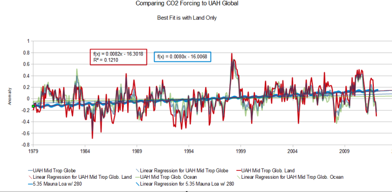
The big question is how much does a change in CO2 have on the atmosphere? The answer depends on the range of change possible. That really hinges on another physical property not yet mentioned, thermal diffusivity. The thermal difusivity of air is roughly its thermal conductivity divided by the product of the density and specific heat of the air. CO2 changes both the thermal conductivity and the specific heat capacity of the air and both in a non-linear manner. The specific heat capacity increase with temperature exponentially, which decreases the thermal diffusivity. The thermal conductivity increases with a decrease in temperature with a maximum value at -20C degrees, then begins to decrease with temperature. In a greenhouse, where temperature, pressure convection are controlled, the impact would be the greatest. In an open atmosphere, convection is not limited, advection, horizontal winds are not limited and pressure is subject to change both locally and with convection. This makes it fairly easy to show greenhouse warming in an experiment, but difficult as all hell in an open system like our atmosphere.

Just to give a real world example of the impact of conductivity and radiant energy flux, consider a radiant barrier or space blanket. Using the US R-value, an air space of 3/4" has an R value of one. Adding a clean, shiny, brand new radiant reflective barrier increase the R-value to three. That would imply that conductivity is at least one third as important as radiant heat transfer between surfaces. It is the transfer between surfaces that creates the convective and latent heats that can transfer energy to another surface at another point in space and time.

BTW, since atmospheric physical properties are related to pressure which is dependent on gravitational force, gravity doe impact climate. But the change in gravity does not appear to produce significant changes in the lower troposphere where we live. It likely does have a small impact in the upper atmosphere, but how much is far from known.

What's up with the Southern Hemisphere?

I love it when statisticians try to explain why some things are significant and others are not. Climate science is heavily statistical with out the benefit of the advice of the heavy weight statisticians.

Global warming should include the entire globe. Half of the global isn't buying into the global warming projected, predicted or fantasized by the climate scientists. Now why would that be?

Probably because the science is missing a few minor details. In order for the greenhouse gases to warm the surface, they must cool some part of the upper atmosphere. Since greenhouse gases cannot product energy, just return a portion of the energy they encounter, the total energy is not changed. For one location to gain more energy, another must lose some energy it would have if it were not intercepted by the greenhouse gases. That is pretty well known, but the point that loses energy is the tropopause and the upper troposphere. If greenhouse gases are warming the surface, the indication of the degree of warming due to extra greenhouse gases would been measurable in the upper troposphere and tropopause.

The Antarctic in winter receives no solar energy. The only energy it can receive would be from the ocean circulation, atmospheric circulation and the upper troposphere/tropopause. For the Antarctic to be cooling in the midst of the most noticeable anthropogenic greenhouse forcing ever, it must be cooling because of the troposphere/tropopause. It should be, because there has been a change in the radiant forcing partially because of additional greenhouse gases. That sounds like a contradiction? Not really.

Since around 1996, the Antarctic temperature has stabilized. That would be an indication that the increase in radiant forcing due to natural and anthropogenic causes has peaked. Should the next prolonged solar minimum reduce global radiant forcing, then the Antarctic will begin to warm. The Antarctic is out of phase with global surface radiant forcing.

With the short length of the satellite temperatures and the unreliable nature of the Antarctic surface temperature measurements, it is impossible to tell accurately, but total global feedback to radiant forcing appears to have caught up with radiant forcing around 1995.

With a prolonged solar minimum, there is likely to be over 0.2 degrees of cooling until the same feed backs that caught up with radiant forcing, fall back to compensate for reduced radiant forcing. Thermal inertia of the ocean upper third is the likely main feed back for this case. What the final temperature will be in indeterminate. There is too much uncertainty in the long term temperature reconstruction to tell what should be average temperature for this period in the history of the Earth.

The inverse relationship of the Antarctic and tropopause to radiant forcing does appear to be the primary driver of one of the internal climate oscillations. More accurate measurement of the Antarctic temperatures should provide insight into future decadal length weather and climate change. However, with all the potential climate perturbations, volcanoes, magnetic field fluctuations, solar cycles and undesirable encounters with objects in space, it is not likely that long term climate is predictable. There is indication though that land use and atmospheric pollution does impact climate, there is still the question of how much by which though.

I would not bet the farm that the statistically challenged climate scientists have much of a handle on the situation, at least, until they can do a better job explaining what is happening in the Antarctic.

Again on Water Absorbs Almost no Solar Radiation

A doubling is Carbon Dioxide is estimated to increase atmospheric absorption of outgoing long wave radiation by 3.7Wm-2. Based on Earth Energy Budgets compiled by NASA, that same atmosphere absorbed approximately 26 PW of out going radiation and 33 PW of solar radiation. PW is Peta Watts of 10 raised to the 15th power Watts per second. 3.7Wm-2 per second with a total surface area of the Earth of 5.1 times 10 raised to the 14th power would be 0.51 PW.

That would be a 1.9PW increase in the outgoing long wave radiation absorbed by the atmosphere increasing the total OLR absorbed to 27.9PW assuming a doubling from the CO2 concentration at the time the Energy Budget chart was created. That extra 1.9PW would be a 7.3 percent increase in the OLR absorbed which would increase the total radiant energy absorbed by the atmosphere by 3.2 percent. Conduction, convection and latent energy is also transferred to the atmosphere. Then total shown on the chart is 111PW, that is all the energy that the atmosphere radiates to space. The doubling of CO2 would initially change that value by 1.7 percent. there is also 10 PW shown of the chart radiated from the surface directly to space, so the total energy radiated to space would be 121PW, so the doubling would initially change that value by one percent.

How much will the solar absorbed by the atmosphere change? How much will the conductive, convective, latent and direct to space energy transfer change?

Of the incoming solar, 33PW is absorbed in the atmosphere and 89PW absorbed by the surface. So of the total 122PW absorbed by the surface and atmosphere, 27% is absorbed by the atmosphere. Of the total 121PW leaving the surface and atmosphere headed to space, 26PW or 21% is from OLR absorbed in the atmosphere. That is a difference of approximately six percent or 7.3PW.

Interestingly, water vapor, which many say absorbs almost no solar radiation, absorbs approximately six percent of the incoming solar absorbed by the surface and atmosphere. That is about 7.3PW versus the 1.9PW of additional absorption expected by a doubling of CO2. That almost negligible absorption by water vapor is nearly four times the expected change from Green House Gas (GHG) Effect change.

With warmer surface temperatures, there will be more moisture in the atmosphere. That increased moisture, water vapor, will absorb more incoming solar. Depending on the altitude of the absorption, the additional energy absorbed will increase convection cooling the surface or block solar absorption at the surface if the additional moisture is near or above the tropopause. Additionally, that increase in water vapor will also absorb more of the returned CO2 radiation, further increasing the rate of convection which is a cooling effect. Water in liquid and gas phase will also absorb more of the incoming solar and the return CO2 return radiation, increasing the rate of convection,m a cooling effect. The water and liquid and ice, is also likely to undergo phase changes in the troposphere, a cooling effect. Lat but not least, in order for there to be more water vapor in the atmosphere, there has to be more surface evaporation, also a cooling effect. The increased surface evaporation would also increase conductive/convective heat transfer from the surface, a cooling effect.

For something that absorbs almost no solar radiation, it sure has a great potential for absorbing solar radiation and changing the impact of returned long wave radiation.

Not Concentric - Not Symmetrical

The Earth is not exactly round and the troposphere is not exactly round either. When modeling things, it is nice to use stuff that is easy. Modelling the greenhouse effect, nice up and down or nice sphere inside a sphere or a box inside a box make the math easier. The nice assumptions might work out with a nice answer or the might work out to a nice mess. Nick Stokes has a blog post on concentric black body spheres used as a basic model of the greenhouse effect. Nick has equations and everything, but the solution boils down to what should be obvious.


In Nick's drawing, which is a lot classier than mine, he shows a section dA to represent the radiant disc used for most black body problems. We assuming the shape of a radiant source, the disc is the best since it is the basic shape used by Planck, Stefan, Boltzmann and the rest of the original gang. The radiation will proceed in all directions, but each of the infinite directions is represented by a small disc, dA. For the concentric circles, representing the sphere in two dimensions, The outer sphere absorbs all of the inner sphere radiation and re-emits 1/2 back to the inner sphere, or circle in the drawing.

If the spheres are not concentric, portions of the outer shape will receive more than others. Also because of the non-uniform shapes, portion of the inner sphere will be missed more by section of the outer sphere. In that case, the outer sphere will receive its own radiation from another point. The absorption will not be uniform, the solution not as simple.

Since all of the inner sphere radiation will be absorbed by the outer sphere, it is easier to concentrate only of the outer sphere. At the apex or point of the outer sphere, less energy is directed to the inner sphere. Near the flatter section, more will be absorbed by the inner sphere.

In this drawing I have added another not exactly concentric sphere, represented as egg shape. The line is exaggerated, but gives the basic idea of what impact the odd shape would produce less return to the inner sphere. All of the energy from the inner sphere would be absorbed by the middle oblique sphere, half of that would be returned and all not returned from the middle oblique sphere would be absorbed by the outer oblique and half of that would be returned to in middle oblique. The middle sphere would return half inward and half outward. The net because of the shape would always be less absorbed by the middle oblique sphere. That difference is likely negligible, but may not be. One of the issues with the greenhouse effect is whether or not it is a small enough error to be negligible. If there are enough spheres, each one would receive less until no radiation would be returned to the center sphere.

What is neat, is no matter the shapes, the outermost sphere or oblique sphere will always return 1/2 of the energy emitted by the inner most sphere. That leaves the only question, what about in the middle oblique sphere? The middle oblique will always return less to the inner at the apex and will always return more at the flatter section. That is pretty much what happens in our atmosphere.


Whether difference is significant seems to be an issue that I personally, do not think should exist. Since water, in various phases increases in concentration below the tropopause to a maximum at the surface and the total density of the atmosphere increase with pressure, it is impossible for downwelling infrared photons to penetrate as easily downward as they can upward. In order for additional greenhouses gases to have the impact estimated in the worst case requires a great deal of creativity.

The first part of the creativity is the simple up/down radiant model. Each GHG molecule absorbs and emits in all directions. By assuming that the curvature of the Earth's surface with respect to the average radiant layer is negligible, the simple up/down model works. The geometry would seem to allow this assumption, but the simple geometry is misleading until one looks at the specific humidity or water content of the atmosphere.

In the Antarctic winter there is the minimum specific humidity found anywhere on Earth's surface. The Zonal Average Moist Potential Temperature in the MIT labweb notes illustrates the issue of assuming geometry is negligible enough for a simple up/down radiant model. From the equator, the high moisture of the upper troposphere forces more down welling long wave radiation towards the poles. This would increase the surface warming in the mid-latitudes, then the symmetry ends. The moist potential temperature drops much more dramatically towards the southerly polar region than northerly. There is no symmetrical polar amplification of additional GHG forcing because there is no symmetrical specific humidity distribution.

With an average annual temperature nearly 30 degrees C lower in the Antarctic, it would require nearly 10 times the estimated GHG forcing to cause a significant increase in Antarctic specific humidity. In the Arctic, less warming would be required for ice free summer conditions, but with the average annual temperature below 250K, it is unlikely that 23 degrees of warming is possible with any reasonable estimate of GHG forcing.

UPDATE: I left Nick a question, what if you add another sphere? here is his answer:

Dallas,
Yes, interesting thought. The "Update" formula extends. The outer shell S3 emits P at emittance P/A3; The second receives irradiance P/A3 from S3 (again it gets the same as it would get at isothermal), total power P+A2*P/A3. And the innermost, S1, receives that emittance P*(1/A2+1/A3) that S2 emits inward (same as outward), which is power P*A1*(1/A2+1/A3). So balancing, S1 emits that plus the source P, with an emittance of P*(1/A1+1/A2+!/A3).

For N spheres, P*(1/A1+....+1/AN)

So like I said, with concentric spheres as a basic model, you would always get the same results. Obviously, our atmosphere is a little more complicated. Since the atmospheric layers are not concentric, the geometry would matter, but the shape of the atmosphere is constantly changing.

Should Nick look into the oblique spheres, he should find that in certain configurations, the spherical assumption is adequate, in others not so adequate. The only relationship I can find that may be consistent, is the Antarctic.

A kick butt model though should notice that the Antarctic is misbehaving by being more stable than expected.

Antarctic Nonsense

In 2009, Eric Steig and company published a paper that made the cover of Nature Magazine entitled, Antarctic Warming. The conclusion of the paper was than the antarctic has been warming at a rate of 0.1 degrees per decade from 1957 to 2006, five decades, 0.5 degrees of warming. The paper received a warm reception from the press, plus plenty of pats on the backs from the crew at realclimate.org.

Not long after the paper was publish, Hu McCulloch, PhD, noticed an error in the confidence interval of the paper published in Nature. That prompted me to write a short article on the quality of climate science and the scientific peer review process, Global Warming and Math Errors.

Not long after I wrote that article, a group of online climate skeptics reviewed the Nature paper finding more errors and ended up publishing their own peer reviewed paper on the Nature paper. If you search for the O'Donnel et. al paper this is the first link you would find, O'Donnell et al 2010 Refutes Steig et al 2009.

The O'Donnell et al paper does not attempt to determine the actual degree of warming or lack of warming in the Antarctic, it merely compares various methods and finds the methodology used in Steig et al 2009 is not very accurate. One of the co-authors of Steig et al 2009 is Micheal Mann, PhD, developer of the iconic Hockey Stick used to provide a visual aid for the proponents of Global Warming. Dr. Mann's statistical prowess has been questioned by many statisticians, and generally found lacking robustness.

In the aftermath of all this scientific squabbling, the temperature record for the Antarctic that still indicates warming of approximately 0.1 degrees per decade in spite of satellite data indicating cooling of nearly the same magnitude for the same period.

The chart above I produced using the surface temperature data available from NASA GISS for the Antarctic region, latitude 64S to 90S in blue and the Satellite data from Remote Sensing Service, RSS for the mid-troposphere latitude 82.5S to 60S. There is a blind spot in the satellite data for the coldest region of the Antarctic, so the two are not exact comparisons. They should be close enough for a reasonable comparison of the trends for the region.

So instead of the Antarctic warming by 0.1C degrees per decade, the satellite seems to indicate that it is cooling by approximately 0.1C degrees per decade. I don't recall the scientists promoting radical economic changes to ward of Global Warming making note of this slight indication of uncertainty.

My question is how much impact would this little mathematical faux pas have on the global mean temperature used to press the need for radical economic changes to ward of Global Warming?

This chart, using the RSS data for the poles and tropics, indicates that there is warming in the Arctic region since 1995, but no warming in the tropics or Antarctic regions of any significance.

Based on this chart using GIStemp versus RSS from 1995 plotted on Woodfortrees.org, the satellite warming from 1995 to present is a little less than half of the warming shown on GISTEMP.

The surface temperature average has been checked by literally thousands of scientists and bloggers. For some reason, the error in the Antarctic still exists and is never pointed out by the scientists advocating radical economic change to combat Global Warming. In fact, the Steig et al paper is still being considered for inclusion in the next version of the IPCC report despite its numerous flaws. Micheal Mann has even published a book on his views of the Climate Wars, where he perceives he is being unfairly criticized by skeptics of his "science". Just about everything that can be done, other than attempting to fix the obvious mistake, is being done.

Personally, I believe I would have to fire a few climate scientists that feel paranoid of the skeptical public should the skeptical public point out their inability to use a basic tool like math. Luckily for some climate scientists, I am not in charge. Should someone that is in charge happen upon this post, hopefully, they will fire a few of the more outspoken scientists that are more concerned with publishing new work, than repairing poor quality work.

Thermohalide Cycles and Antarctica

The impact of Antarctica on the thermohaline circulation of the oceans has been plauging me for some time. Most of the problem is the lack of quality data in the Antarctic and the length of the instrumental temperature record. The chart above appears to be a key part of that puzzle. By using the RSS Antarctic region mid-troposphere temperature data, I appear to have found a conflict with the surface temperature average. The Antarctic according to RSS is cooling and has been cooling for some time.

This reconstruction of temperatures in southern South America, from the NOAA paleo website, provided by R. Neukom1, J. Luterbacher2, R. Villalba3, M. Küttel1,4, D. Frank5, P.D. Jones, M. Grosjean1, H. Wanner1, J.-C. Aravena7, D.E. Black8, D.A. Christie9, R. D'Arrigo10, A. Lara9,11, M. Morales3, C. Soliz-Gamboa12, A. Srur3, R. Urrutia9, and L. von Gunten1,13., may indicate that current cooling in the Antarctic started around 1945, hard to tell. There appears to be general cooling for the entire length of the reconstruction with general warming for the last half.

Since I suspect some influence from the 22 year Hale solar cycle, the above plot compares the SSA reconstruction with the Jacoby et. al Taymyr Peninsular reconstruction from Siberia. This shows that both have similar longer term pseudo cycles and there is roughly a 30 year lag between the two polar regions. There is also a change in the correlation starting around 1931. This change is likely due to agricultural and/or industrial expansion in the northern hemisphere which did not occur to the same extent in the southern high latitudes.

Nearly lost in all the noise is the lag between the two polar regions. Since radiant forcing is much more rapid than ocean heat uptake or loss, the Antarctic is a major source of the deep ocean heat loss and that there appears to be little change in the Antarctic due to the efforts of mankind, I would suspect that the lag is related to ocean heat content. That suspicion may be a reach, but the cycle length of the Pacific Decadal Oscillation agrees rather well with the lag.

The physical cause of the lag is somewhat complex. If it were in better agreement with the solar cycle, it would have already been well documented. Since it has not been well documented, it is open to theory.

The best explanation I can find for the lag and the long term pseudo oscillation is the change in atmospheric conduction caused by Carbon Dioxide variation associated with general warming and cooling combined with the tropopause altitude/temperature variation cause by the radiant forcing variations of the same greenhouse gases.

In order to warm the surface, the greenhouse gases must cool the tropopause. Since the Antarctic is closely related to the conditions of the tropopause, that cooling, out of phase with surface warming, increases deep ocean heat loss in the Antarctic region waters.

With the apparent error in the Antarctic surface station data, this unique feedback relationship would not be obvious. Also because of limited instrumentation, the relationship of the Antarctic geomagnetic north pole and synchronization with the solar magnetic field impacting the efficiency of ocean heat loss to the Antarctic atmosphere, is not easily verified.

Time though will resolve all of the issues. In the mean time, simple options to avoid excessive Northern Hemisphere warming are available.

http://tenaya.ucsd.edu/~tdas/data/review_iitkgp/2010JD013949.pdf

The average length of the thermohaline cycle appears to be 236 years, BTW. Much better paleo reconstructions would be needed to confirm that, but focusing a little more on regional reconstruction should help resolve that issue. I believe that a newly launched polar orbital satellite should make some head way on the geomagnetic issue. In any case, that is the new installment in my theory of the ice ages.

What do You Choose to Believe?

The Medieval Warm Period was only a regional event. If that is your belief, then warming in the 20th century has to be abnormal and require explanation. The chart above is my mine using the South American Temperature Reconstruction of R. Neukom1, J. Luterbacher2, R. Villalba3, M. Küttel1,4, D. Frank5, P.D. Jones, M. Grosjean1, H. Wanner1, J.-C. Aravena7, D.E. Black8, D.A. Christie9, R. D'Arrigo10, A. Lara9,11, M. Morales3, C. Soliz-Gamboa12, A. Srur3, R. Urrutia9, and L. von Gunten1,13. I don't know any of those people, but they seem to believe that the Medieval Warm Period was not a regional event. Looking at their data, South America has been warming since the 1400s. South American may have had its MWP, just a little out of sequence with some parts of North America.

" Although we conclude, as found elsewhere, that recent warming has been substantial relative to natural fluctuations of the past millennium, we also note that owing to the spatially heterogeneous nature of the MWP, and its different timing within different regions, present palaeoclimatic methodologies will likely "flatten out" estimates for this period relative to twentieth century warming, which expresses a more homogenous global "fingerprint." Therefore we stress that presently available paleoclimatic reconstructions are inadequate for making specific inferences, at hemispheric scales, about MWP warmth relative to the present anthropogenic period and that such comparisons can only still be made at the local/regional scale." That quote is by D'Arrigo, R.; Wilson, R.J.S.; Jacoby, G.C. from their abstract in the D'Arrigo et al. 2006 Northern Hemisphere Tree-Ring-Based STD and RCS Temperature Reconstructions.

If you focus on regions, your belief would be that AGW is not as much of a factor as natural warming, recovery from colder times caused by the Little Ice Age. If you look at the massive land use changes in the Northern Hemisphere, nearly 3% of the total surface area of the globe converted from wilderness to human habitat, you would assume there is some Anthropogenic warming that is beneficial and needed.

If you focus on CO2, you can determine that CO2 is causing global warming and that it is bad, because it is unintentional.

If you look at everything objectively, you may believe that some warming is good, some is natural and some may be bad, but we really don't know how much of any warming is due to any specific cause.

To my mind, having any opinion other than we don't really know, requires belief, not science.

Even More Calibrating Imperfection

What happens when you compare the Atlantic Multidecadal Index, Taymyr Peninsular tree ring reconstruction, the Central England temperature record, Volcanic Explosion Indexs and a few Siberian instrumental records? You crash the heck out of Opensource spreadsheets! You do get some interesting stuff though.

One of the biggest problems was that the AMO and the Taymyr had a pretty good correlation but a few things that looked goofy. The CET also match in a lot of places, but missed the boat in quite a few. So I averaged the AMO and the CET and compared to the Volcanic data available from the Global Vulcanism Program. The older major eruptions had a lot of estimates and questions on the dates. I just used the estimated date and best guess for the magnitude of the eruptions and used a 17 year moving average. Pretty crude, but it gives a rough idea of the impact of the Vulcanism on the AMO, mainly for the equatorial eruptions and the CET (March-April-May)/Taymyr for the northern hemisphere smaller eruptions.

The Average (1) curve is the average of the anomalies for three Siberian surface stations, Ostrov Dikson near Taymyr, Turuhansk, a little south of Taymyr and Pinofilovo which is in the major farming region of Siberia. The Pinofilovo station is plotted by itself to highlight how it tends to break the trends starting in around 1900. Far from conclusive that agricultural expansion is a major cause of the Siberian warming, but getting much closer to being somewhat convincing.

Russian records are pitiful, but there was a general expansion into the Siberian region at around 1900 and another push starting in the late 1950s. Russian production per hectare was about 30% to 50% less than in the US even though they exported more than the US in the early 1900s. One report for 2011 stated that Russian was planting 500,000 hectares of winter wheat. That is only 5,000 kilometers squared, but that should be about half of the acreage set aside for winter wheat allowing for crop rotation. There is also considerable barley, sugar beets and rye, for pasture and rotation, with about 8% to 10% of the total land area of Russia devoted to arable land. This is a smaller area than in the US but near the area in Canada used for grain crops. Canada also has a higher temperature trend in its interior farm belt than the global average.

The major albedo impact of large scale grain farming is two to three months per year, planting and harvest, where the land can absorb around 20Wm-2 more than it would in a virgin state. Since Russian records are so bad, I will have to use Canadian lands near the same latitude and attempt to interpolate the impact to Russia.


More: From Wikipedia, Total land under cultivation, 17,298,900km^2 or 11.61% of the land surface area. Russia, 1,192,300km^2, Canada, 474,681 km^2, United States, 1,669,302 km-2 and China, 1,504,350 km-2 totaling 4,840,633 km^2 which is 3.25% of the land surface area or 0.95% of the total surface of the globe. This doesn't include the second largest agricultural country India as I am mainly interested in impact above latitude 45 degrees North. This should include Kazakhstan and the Ukraine, with nearly 600,000 km^2, but I intend for their area to offset the southern portion of the US.

On a yearly average, the northern latitude albedo change due to agriculture would have to produce slightly over 1 Wm-2 to offset 50% of the estimated warming due to increased atmospheric CO2. Since the major impact of agriculture is only during the growing season and peaking in only about 2 months of that period, the impact during that time would need to be approximately 6 Wm-2.

The image from Wikipedia above indicates that is not unrealistic.

Calibrating Imperfection?

The Taymyr Peninsular in Siberia has a reasonably long Russian Larch tree ring proxy compiled by Jacoby and gang which is dated 2006 and archived on the NOAA paleo site. The series ends in 1970 because Jacoby and gang determined that the proxy diverged from temperature starting in that date.

Ostrov Dikson is a small Russian town located on an island at the west side of the Taymyr Peninsular. It has an airport and a temperature record starting in 1918. There are three data points for the March through May average that are missing. I interpolated those for the average of the preceding and following values just for the spread sheet.

Using the period of overlap, 1918 to 1970, I shifted the Ostrov series so that the average of the overlap period aligned with the Taymyr data. The yellow mean for Taymyr and the green mean for Ostrov are shown on the chart.

The mean for Ostrov Dikson from 1970 to present is shown in red and is approximately 0.6 degrees higher than the 1918 to 1970 mean. The full series mean of Taymyr in blue, is about 0.4 degrees lower than the 1918 to 1970 mean.

The best average growth rate for the Taymyr series is near the 1918 to 1970 mean, with 1918 to 1950 being close to the optimum growth rate for the series. That should indicate than the period between 1918 and 1950 to 1970 should be the near the optimum conditions, temperature, precipitation etc. for the type of tree.

This chart shows the entire period of the Taymyr tree ring series.

Above I have added the central England temperature centered on the 1918 to 1970 period so that all three series have a common base line. The match, considering trees are not thermometers is pretty good. With the CET series add, there are periods were temperatures above the mean correspond with reduced tree growth and period where when temperatures are below the mean there is reduced tree growth. While the tree rings series do not provide a great deal of temperature information, they do have potential to provide more information about what is average global temperature, at least as I interpret the data.

Note: the CET data is also March through May.