The Best Place to Start is at the Beginning

The Antarctic Circumpolar Current is the main driver of the deep ocean currents.  The chart above was borrowed from Wikipedia.  Sailors know that the winds and seas in the southern latitudes from 40 to 60 south are not for the faint of heart.  Those high winds drive the seas that creates the circumpolar current.  With the higher average surface wind velocity and little land mass to deflect the current, huge amount of energy are exchanged between the cold ocean waters and the atmosphere.  This region is the thermal regulator of Earth's climate.

Update: The Flow of the Antarctic Circumpolar Current through the Drake Passage is estimated at 95 to more than 134 Sverdrup which is 10^6 cubic meters per second.  The Gulf Stream current off Florida is estimated at 35 Sverdrup.  Somebody asked so there is the best answer I could find.  

This graph is 131 month sequential standard deviations of the UAH lower troposphere regional temperature anomaly.  The two curves with the least deviation are the southern extend and the southern extent oceans.  The low standard deviation indicates the stability of the temperatures of each region.

This chart is the sequential standard deviations of the GISS LOTI regional temperature anomaly.  Again the least deviation is in the 64S to 44S latitudes.  Finding a regional so stable in a chaotic climate and weather system is exceptional.  That stability is useful in determining the best fit to other data, especially paleo climate proxy reconstructions.  Unfortunately, most paleo climate reconstructions end in inconvenient times.  To determine where those reconstructions best "fit" with newer instrumental data can be challenging.  By using the most stable instrumental regional data and working back towards the noisier regions, it is posible to have greater confidence in the "fit" or splice of the instrumental to the paleo reconstructions.

This is an example of splicing the 64S-44S GISS LOTI temperature to the Southern South American temperature reconstruction by Neukom et al. 2010.  My apologies for misspelling the name on the chart, the link should soothe any perceived slight.  With this "splice", the instrumental data fits well with the temperature anomaly of the paleo reconstruction.  I have not include any error bars because at this time the degree of uncertainty is not easily determined.  The centered 5 year smoothing applied to each data series is intended to not overly smooth any information that they may contain, just eliminate some of the noise in each.  The object is to determine an appropriate baseline to start rebuilding a better picture of past climate with other regional reconstructions.

Perfectly "slicing" imperfect data is impossible.  Using the 1979 to 1990 inclusive satellite era baseline, p.b.l. to combine with paleo climate reconstructions typically ending before 2000, does appear to allow better combination of the different types of data.  Sea level data and reconstructions would tend to be less variable, allowing not only a simpler "splice" but qan indication of the differences in sensitivity of the differing data sets.  The chart above combines HADSST2 southern hemisphere and the UAH Southern Extra tropics lower troposphere data.  Because of the lower density of the atmosphere where the average UAH temperature is determined, there would be more variability in the temperature.  The thermal mass of the oceans naturally smooth the HADSST2 data and the Neukom reconstructions using various proxies would tend to be more noisy.  In the chart above, the 1900 to present time period is highlighted to show the quality of fit using the p.b.l. base period.

Starting the plot in 1250 and inserting the mean value of the UAH data in green and the mean value of the full SSA reconstruction starting in 900 AD, the mean temperature of the southern extra tropics would be approximately 0.5C greater than the mean temperature of this region.  The absolute value of the SSA reconstruction may be uncertain, but the mean should be useful for combining other longer term reconstructions.

One of the issues with combining paleo reconstructions is how much resolution is useful.  This chart combines Cook et al 2000 Tasmania with the Neukom et al. Southern South America and the GISS LOTI 44-64S instrumental.  Using the same p.b.l with 5 year centered smoothing there is a good deal of noise.  The mean value lines for each series is included showing that the range of means is from about -0.3 to -0.5C.  Despite the noise, that is a remarkably close range of mean for 4000 years of climate.  Of course the reconstructions may have issues.  By increasing the smoothing period, there would be less noise reducing the peak values.  Smoothing them enough, we would have a hockey stick with current temperatures about 0.4 to 0.5C higher than the past mean, but that is already shown.  Ideally, any more smoothing would match the natural smoothing of averaging the surface temperature instrumental.

Expanding the Time Frame:

Extending past climate beyond 900 AD is a bit of a challenge.  Since the Ice Ages would have a much more pronounced impact near the poles and at higher elevations, tropical reconstruction would give a better indication of ocean temperatures but not global temperatures.  The southern high latitudes may have been frozen to some point.  Antarctic sea ice advance could have shut down or greatly reduced the Antarctic Circumpolar Current.  So this next step is a bit of a guess.

The Tierney et al. 2008 Lake Tanganyika surface temperature reconstruction is added with the darker green full reconstruction period mean value and the 10000BC to 695AD section in the lighter green with its mean value.  By subtracting 0.6C from the mean of the overlap period with the Tasmania reconstruction, we get the orientation shown.  It could be higher or lower, this is just a rough fit.

Here is the full reconstruction just for completeness.  There are a few other reconstructions of past temperature that generally agree with this rough orientation.  The Nielsen Southern oceans SST for the Holocene for example has what appears to be a longer term oscillation out of phase with the Lake Tanganyika reconstruction.

The range of temperature swing is larger, consistent with Antarctic Circumpolar Current changes driving climate, but will require some deeper digging to relate to global conditions since according to this, the first part of the Holocene was a severe southern extratropics near ice age following an ice age normal temperature range.  Interesting.

During the modern era, the instrument data provides hints of the different oscillations and dampening constants of the hemispheres.

By selecting different smoothing and comparing regions, like the Tropics and Extra Tropics above, you can get a reasonable picture of the heat transfer between the regions of the oceans.  The satellite series started with a small volcanic event that impacted the northern hemisphere.  By 1991, the Southern na Northern Extratropics appeared to have been equalized only to that the Pinatubo eruption in 1991 drive northern hemisphere temperatures down again.  The extra tropics reached the same capacity again in 1996 setting the stage for the temperature equivalent of a rogue wave in the 1998 Super El Nino.  Since then, the temperatures a falling in a dampened manner with various harmonic synchronization generating smaller El Nino and La Nina events.  Much longer term oscillations are likely which are probably generating the "noise" in the paleo climate reconstructions.

The 1991 Pinatubo eruption provided a nice perturbation to the ocean thermodynamics.  Following Pinatubo, there was a self organizing of the internal oscillations that produced the nifty 1998 Super El nino.  Since the rate of heat transfer is different between the hemispheres, the dampening is a bit difficult to follow, but clear enough for the cyclomanic geeks in the crowd.  Since I don't have the more accurate 24N to 44S main thermal capacity of the oceans, the tropics will do for now.

The UAH tropical oceans are in yellow for this plot.  Comparing the HADSST2 hemisphere data you can follow the somewhat chaotic oscillations back in time.  Remember that the Southern Hemisphere contains only about 1/3 of the land mass of the Northern Hemisphere and the Antarctic continent makes up a substantial portion of the Southern Hemisphere land mass.  For the instrumental period, we have had remarkable stable temperatures well within the "normal" range of an interglacial as far as the oceans are concerned.

With the exceptions of the polar regions, there is no real reason for the average temperature of the oceans to change much during glacial/interglacial climates.  The total energy of the atmosphere would change much more than the total energy of the oceans since sea ice advance insulates the polar oceans.  The main caveat to that is the Antarctic Circumpolar Current which is the main heat sink of the oceans.

Once Antarctic sea ice extent increases to the South American peninsular, the efficiency of the ocean/atmosphere heat transfer most likely to released energy to space would be reduced.  This would likely increase the heat loss at the northern pole increasing high latitude precipitation where the mass snow and ice could accumulate at high elevations, not only in the Northern Hemisphere, but in all higher elevations of the Earth.  Oddly, the accumulation of snow on the more permanent Antarctic sea ice would likely be a significant driver of reduced global sea level where the sea ice was "fixed" or landed.  The building and breaking of these Antarctic fixed ice accumulations could produce some interesting "Red Herrings" in the iconic Antarctic ice core history of global climate.    I'll have to search for a few of those anomalies.

The tropical oceans reconstruction above for 400,000 years compiled by Herbert, T. D. et al. have different calibration periods.  Instead of attempting to average exactly, the lower glacial temperature anomaly is estimated with the blue bar and the interglacial average estimate is the red bar.  That implies a range of about 3 C or +/- 1.5 C which is pretty consistent with the +/-1 C control range likely impsed by the freezing points of salt and fresh water.  The most stable of the reconstruction is the tropical Atlantic which can be directly compared to the Western Caribbean reconstruction of Schmidt, M. W. et al. in the next segment.



Anywho, to be continued.

I wasn't up to the Caribbean yet, but since I got into a discussion on the Milankovic Cycles that don't quite match the ice ages because ice ages are not all the same, I just threw this in for the moment.  I hope it does give away the ending :)  Schmidt, M.W. et al. 2006 is on the NOAA paleo site if you are interested.

The Schmidt et al. Western Caribbean is one of many longer term reconstructions not often mention in climate science.  By combining the Western Caribbean with southern oceans reconstruction and the Lake Tanganyike lake surface temperature reconstruction you can see why.  There are longer term internal ocean oscillations which tend to confuse most folks.  The southern oceans are the main heat sink for the planet, but they don't catch up with global heat capacity changes quickly in all cases.  That produces the internal oscillations on all time scales.

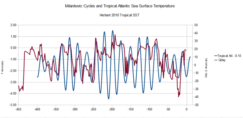
The tropical Atlantic ocean and the western Caribbean have a better correlation to energy input.  This plot is the Milankovic solar cycle model with the Herbert et al. Tropical Atlantic SST reconstruction.  This is a fairly good fit with the typical miscues due to volcanic and other internal impacts which have to be sorted out.  The time scale above is in thousands of years, so techically we would be in what is called a Glacial Episode.  With not unoccupied land mass to accumulate glacial mass, there is not good likelihood of entering a glacial period.  That is an impact of Antropogenic Global Warming caused mainly by land use and our ability to clear snow.