Clouds, ENSO, Adjustments and Feedback

I love when the conversation turns to clouds and whether they are a positive or negative feedback.  Clouds are both.  Whether they are a "net" positive or negative feedback depends on where they change.  Since they are not "fixed" I doubt there is any definitive proof they are anything other than a regulating variable since they can swing both ways.

At higher latitudes clouds are most likely positive feedbacks.  Winter clouds tend to let the cloud covered region get less cold.  In the tropics, clouds tend to keep areas from getting too warm.  The battle ground should be the mid latitudes.

Since most of the energy absorbed is in the tropics, knowing how well the tropics correlated with "global" temperature would be a good thing to know so that you can get a feel for how much "weight" to place on the "regional" responses.  With the exception of the 21st century, the "Global" temperature have followed tropical temperatures extremely closely.  Now it would be nice to just compare changes with cloud cover with changes in tropical temperature right?

Nope, the cloud fraction data sucks the big one.  Since that data sucks so bad you are stuck with "modeling".  You can use a super doper state of the art climate model or you can infer cloud response based on logic.  Both are models since you are only going to get some inferred answer, the logic just cost less.

Logic: Since warmer air can hold more moisture than colder air, all things remaining equal, there would be an increase in clouds with ocean warming.  If clouds were "only" a positive feedback to surface warming, the system would be unstable and run away.  Simple right.  You can infer clouds must have some regulation effect on tropical climate or there would be no tropical oceans.  They would have boiled away or be frozen.

That logic obviously has limits.  There is more to the globe than the tropics and there is and has been warming in the tropics.  Could it be we have reached a tipping point that will change millions of years worth of semi-stable temperatures?

This is where paleo data could come in handy.

 I use this Oppo et al. Indo-Pacific Warm Pool quite often because it agrees well with the tropical oceans which agree well with "global" temperatures and is backed by the simple logic that the oceans wag the tail.  So provided the IPWP does "teleconnect" with "global" climate, things look pretty "normal".  There was a cooler period that Earth is recovering from and now she is back into her happy zone.  There are absolutely no guarantees that is the case, just evidence that it could be.

Since "global" climate follows tropical oceans so closely except for that little 21st century glitch,  there probably isn't much more to worry about in the tropics.

If I use the not so elaborately interpolated GISS data, the 250km version instead of the 1200km version, there isn't any glitch to be concerned about.  Climate suddenly gets a lot more simple.  The tropical oceans have been warming for the past 300 years to recover from the little ice age and now thing are back to "normal" for the past 2000 years.  CO2 has some impact but likely not anywhere near as much as advertised.  That would imply clouds/water vapor are not as strong a positive feedback as estimated.

Well, simple, really doesn't cut it in climate science.  There are a lot of positions to fill and mouths to feed so complexity leads to full employment and happy productive climate scientists.

That means "adjustments" will be in order.  Steven Sherwood, the great "adjuster", has a paper that explains what is required to keep climate scary enough for climate scientists to help save the world from itself.  Part of the "adjustments" is removing or managing ENSO variability and volcanic "semi-direct" effects so that the monstrous CO2 signal can be teased out of the "noise".  Then, clouds will be a net positive feedback and water vapor will drive climate higher and we will finally see the ominous TROPICAL TROPOSPHERIC HOT SPOT!  Then finally, it will be "worse than we thought".

Think just for a second.  If the tropical oceans "drive" global climate, and ENSO is a feather of the tropical oceans, why in the hell would you want to remove the climate driver?  Because it is inconvenient.  Natural variability (read ENSO) cannot POSSIBILITY be more than a tiny fraction of climate because my complex models told me so.  According to a few trees in California and Russia, that Oppo et al. reconstruction has to be total crap because climate never varied one bit until this past half century once we got the surface stations tuned and adjusted to fit the models that are tuned and adjusted to match our theory that CO2 is tuning and adjusting climate.  Can't you thick headed, Neanderthal, deniers get it that we are "climate scientists" and know what we are doing!!

Frankly, no.

Added;  In case you are wondering, there is a 94.2% correlation between annual ERSSTv3b tropical SST and GISS 250km "global" temperatures.  The tropical oceans are about 44% of the global area.  The 11 yr average difference between the two is +/-0.1 and close to +0.2/-2.8 annually.  While long range interpolation does produce a more accurate "global" average temperature it doesn't produce a more accuarte "global" average energy due to very low temperature anomalies having the same "weight" as much higher energy tropical anomalies.

From the Basics- the 33 Degree "Discrepancy"

The 33 degree discrepancy is the starting point for most discussion on the Greenhouse Gas Effect.  It basically goes like this:

The Earth receives 240 Wm-2 of solar energy which by the Stefan-Boltzmann Law would have a temperature of 255K degrees,  The surface of the Earth is 288K degrees which by the Stefan-Boltzmann Law would have an energy of 390 Wm-2.  The differences 33C(K) degree and 150 Wm-2 are the Greenhouse Gas Effect.

Sound very "sciency" and authoritative like it is carved in stone.  It is actually a logical statement.  If this and if that then this.  So there are several hidden assumptions.

First, the Stefan-Boltzmann law has an uncertainty of 0.924 which is a bit more of a low side instead of a plus or minus type of uncertainty.  That is important to remember because a lot of statistics assume a "normal" distribution, +/- the same amount around a mean, to be accurate.  The S-B correction is related to efficiency which cannot exceed 100% so 0.924 implies you can "expect" around 92.4% efficiency.  I am sure many can argue that point, but that is my understanding.

So using that uncertainty "properly", both sides of the 33C discrepancy should have -0.76% error bars included in there some where.  I have never seen that displayed on any AGW site.  So for the solar energy received you should have 240 Wm-2 to 222 Wm-2 or about 18 Wm-2 of slop.

That "slop" may be due to a number of factors, but since the 33C discrepancy assume a constant reflection, there is a good chance that the two are inextricably inter related.  There is no "perfect" black body and low angle reflection is likely the reason.  We can get flat surfaces to behave like 99.9999.. percent black bodies, but most objects are not perfectly flat.

Now this large error range was actually included in one of the more recent Earth Energy Budgets by Stephens et al.

Right at the bottom by Surface Imbalance is a +/-17 Wm-2.  Now that error range is based on a large sampling of guestimates, not the basic S-B law, but it is pretty amazing to me how well the old guys included uncertainty.  Now you could jump in and say, "but that is a +/- error range!"  True, but it is based on guestimates.  You could rework the budget so that you could reduce that range to about half or around +/-8.5 Wm-2, but you are going to find it hard to get below that range.

The Mysterious Land Amplification Issue

I notice the odd land amplification in the Northern Hemisphere between latitudes 30 and 90 North a long time ago.  The Berkeley Earth Surface Temperature project pick up on it but by and large it is pretty much ignored.  Originally, I was pretty certain it had to be due to land use and/or surface station impacts due to land use, but there isn't really anyway that I have found to make a convincing case.  So it is still a mystery to me.

In the chart above I tried to highlight the situation.  Excluding the poles since the SH coverage really sucks, all of the globe pretty much follows the same course.  The highly variable region from 30N-60N really makes a jump with the 1998 El Nino.  It looks like it tried to jump prior to Pinatubo, but got knocked back in line for a few years.  Southern Hemisphere and equatorial land temperature don't even come close to making the same leap.

The RSS lower troposphere data makes a similar leap but with about half the amplitude.

Berkeley Earth Tmax makes the big leap.

Berkeley Earth Tmin makes about the same leap though Climate Explorer picked a different scale.  That should reduce the chances that it is a UHI issue.  Even though there are some issues with Tmin, a land use cause should have more Tmax influence than Tmin if it is albedo related in any case.  That could also put Chinese aerosols out of the running.

Playing around with the Climate Explorer correlation option, the amplification seems to correlated with the growing season so it could be related to agricultural land use or the more variable vegetation related CO2 swings.  DJF have the worst correlation which for this time frame, 1979 to present would be consistent with the change in Sudden Stratospheric Warming events and greater Arctic Winter Warming.  Climate Explorer has limited series for their correlation option and I haven't attempted to upload any of my own yet.


So there is still a mystery there for me.  This post is just to remind me of a few things I have looked at so perhaps I will stop recovering the same ground and possibly inspire some insomniac to join in on the puzzle.

The Never Ending Gravito-Thermal Effect

I have my issues with "ideal" models, they are useful but rarely "perfect.  So when an "ideal" model/concept is used in a number steps during a derivation, I always look for how wrong can that be.  I may be a bit of a pessimist, but that is something I consider "normal" because virtually nothing is absolutely 100% efficient.  The Gravito-Thermal "Effect" seems to boil down to interpretation of an ideal kinetic temperature concept used to formulate the ideal gas laws.

Hyper-Physics has a very nice explanation of Kinetic Theory.

 The force exerted by any number of gas molecules can be simplified by assuming "perfectly" elastic collisions with the walls of a container, ignoring collisions with other molecules, so that kinetic energy is *exactly* equal to;

If you include gravity, the force exerted upwardly would always be less than the force exerted downward.  When you have a lot of molecules and a small distance between top and bottom, the difference is negligible.  The greater the distance, the more likely there will be some significant difference in the force applied to the top and bottom of the "container" which is the Gravito-Thermal effect.  If you have a scuba tank, don't expect to see any temperature difference.  If you have a very tall tank with very few molecules, there is a likelihood there will be some "kinetic temperature" difference between the top and bottom.  Kinetic temperature is in quotes because what it really is is average applied force.  That is the very first assumption made in the derivation.

So if you install a pressure sensing plate, like a thermocouple at the bottom and top of a very tall container they would measure different applied pressures even though everything else in the container remains constant.

Remember though that Kinetic or translation temperature doesn't include anything but three directional degrees of motion or freedom.  Real molecules have more tricks up their sleeve that can produce radiant energy transfer and stored energy as in potential or enthalpy.  The ideal gas concept promotes conduction which is related to diffusion in a gas, to the grandest of poobahs of heat transfer.  In the real world conduction is gases is pretty slow and not all that efficient.

Most folks would drop the subject about now and admit that there would be a "real" temperature difference in some cases, but there are so many other "real" issues that have to be considered that any further discussion of the Gravito-Thermal effect based on an ideal gas is about the largest waste of time imaginable.  Not so in the world of academia where every nit is a potential battle ground.

Key points for them wishing to waste their time would be is gravity an "ideal" containment since gravity doesn't produce heat, it is the sudden stops that produce the heat. If the gas has the "potential" to whack something and doesn't, it doesn't transfer an force so it is not producing the heat which would be the temperature in the case of an ideal gas.

Some of the more creative seem to think this "ideal" case will result in a fantastic free energy source that will save the world.  I am not sure why "saving the world"  always seems to boil down to the more hair-brained of concepts, but that does appear to be the tendency.  A neutron busting the hell out of a molecule produces much more energy which has a proven track record of providing usable energy when properly contained and not embellished with Hollywood fantasy super powers.  But as always, one persons dream is another's nightmare. Even if all the fantasy inventions worked, there would still be a need for someone to save the world from perfection.

During the last "debate" I mentioned that for a rotating planet, the maximum velocity of the molecules in the upper atmosphere would be limit by the escape velocity or speed.  So even ignoring all the other minor details, gravity has containment limits which would be temperature limits.  Earth for example loses around 3 kilograms per second of hydrogen in spite of having a geomagnetic shield that helps reduce erosion of the atmosphere and there are molecules somewhat suspended in pseudo-orbits of various duration depending on their centrifugal force versus gravitational force.  Centrifugal and gravitational forces again don't produce heat until that energy is transferred.  So a cluster of molecules could be traveling along at near light speed, minding their own business, having a "local" temperature that would tend to change abruptly if the clusters whacks another cluster.  Potential energy is not something to be ignored.

Speaking of potential energy, during the last very long discussion, the Virial Theorem made a showing and I was chastised for mentioning that the VT produces a reasonable estimate.  This lead to another *exact* discussion where if you force the universe to match the "ideal" assumption required, mathematically, the "solution" is *exact*.  Perfection doesn't really exist sports fans.  Every rule has its exception which is what makes physics phun.  In "ideal" cases those constants of integration are really constants but in the real world they are more likely complex functions.  More often than not, assuming the constant is really constant is close enough for government work, but a smart engineer always allows for a bit of "slop" or inefficiency if you prefer.  Some scientist tend to forget that, so IMHO, it is always nice to have an engineer on hand to provide reality checks.

What was interesting to me about the whole discussion was how the universe tends to prefer certain version of randomness more than others.  For the Virial Theorem, T=2*Tp or kinetic energy is equal to 2 times the potential energy.  So Total Energy is never equal to a perfectly isothermal of maximum entropy state.  Since the universe is supposed to be moving towards an ultimate heat death or true maximum entropy some billions and billions of years in the future, potential energy should slow be reducing over time.  That would make the Virial Theorem a good estimate for the way things are now which should be close enough for a few billion generations.  So for now, potential is about 2/3 of total so the things physical in the universe should prefer a ratio in the ballpark of 1.5 to 2.

If you have read some of my older posts, V. M. Selvam likes to use the Golden Ratio of ~1.618... in her Self Organizing Criticality analysis and Tsallis among others finds similar common ratios for "stable" systems.  Nothing is required to be "stable" in dynamics forever so "preferred state" is probably a better term than "stable state".  When things get close to "equilibrium" 2nd and 3rd order influences can tend to ruin that "equilibrium" concept which is joined at the hip with the entropy concepts.

Boltzmann's concept of entropy would then be a bit too ideal, which started the whole Gravito-Thermal debate to begin with.  Gibbs, Tsallis and many others have functions, intentional or not included in their definitions of entropy to allow for the "strangeness" of nature.  Nature probably isn't strange at all, our ideal concepts are likely the strangeness, which is apparent in any debate over the Gravito-Thermal Effect.


Update:  Since I started this mess I may as well link to John Baez and his Can Gravity Decrease Entropy post.  He goes into more detail on the Virial Theorem on another post in case you are curious.  The main points, IMHO, is that a gravitationally bound system cannot ever really be in "equilibrium". with its surrounds and the basic requirement for an isothermal or even an adiabatic system is the need for some "real" equilibrium.  Boltzmann's entropy is a attempt to maximize "within a volume", that f=ma issue and a system bounded by gravity is trying to increase entropy by decreasing potential energy, i.e. compressing everything to create heat/kinetic energy.  A gravitationally bound system will either completely collapse or portions will boil off.  The Ideal kinetic model maximizes entropy by not allowing anything to boil off.

.  

Why do the "Alarmists" Love Marcott et al.?

Because it looks like what they want.  The Marcott et al. "hockey" stick is spurious, A result of a cheesy method, not including data that was readily available and a few minor date "correcting" errors.  The authors admit that the past couple of hundreds years are "not robust" but even highly respected institutions like NOAA include the "non-robust" portion as part of a comedic ad campaign.

I don't think that self-deception is actionable since that is just part of human nature, but when the likes of NOAA join the moonbeams, it can become more than comical.  Unlike the Mann hockey stick where inconvenient (diverging) data was cutoff, Marcott et al. just didn't dig a bit deeper to find data that didn't "prove" their point.  A great example is the Indo-Pacific Warm Pool (IPWP).  Oppo et al. published a 2000 year reconstruction in 2009 and Mohtadi et al. a Holocene reconstruction of the IPWP in 2010.  If you compare the two, this is what you "see".

The sparse number of data points in Mohtadi 2010 picks up the basic rough trend, but the Oppo 2009 indicates what is likely "normal" variability.  When you leave out that "normal" variability then compare to "normal" instrumental variability, the instrumental data looks "unprecedented".

Since the lower resolution reconstructions have large, on the order of +/- 1 C of uncertainty and your cheesy method ignores the inherent uncertainty of the individual times series used, you end up with an illusion instead of a reconstruction.

The funny part is that normally intelligent folks will defend the cheesy method to the death instead looking at the limits of the method.  The end result is once trusted institutions jumping on the group think bandwagon.

The data used by Marcott et al. is available on line in xls format for the curious and NOAA paleo has most of the data in text or xls formats so it is not that difficult to verify things fer yerself.  Just do it!

My "just do it" effort so far has the tropical ocean temperatures looking like this.

The tropical oceans, which btw are the majority of the oceans, tend to follow the boring old precessional orbital cycle with few "excursions" related to other climate influencing events like Ice dams building/breaking, volcanoes spouting off and the occasional visit of asteroids wanting a new home.  That reconstruction ends in 1960 with some "real" data and some last known values so there is not so much of a "non-robust" uptick at the end.  It only includes "tropical" reconstructions and there are a few more that I might include as I find time and AD reconstructions to "finish" individual time series.

The Problem with Changing your Frame of Reference from "Surface" Temperature to Ocean Heat Content

The few of you that follow my blog know that I love to screw with the "geniuses" aka minions of the Great and Powerful Carbon.  Thermodynamics gives you an option to select various frames of reference which is great if you do so very carefully.  Not so great if you flip flop between frames.  The minions picked up the basics of the greenhouse effect fine, but with the current pause/hiatus/slowdown of "surface" warming, they have jumped on the ocean heat content bandwagon without considering the differences that come with the switch.

When one theorizes about the Ice Ages of Glacial periods, when the maximum solar insulation is felt at the 65 north latitude, the greater energy would help melt snow and ice store on land in the higher northern latitudes.  (Update:  I must add that even the shift to maximum 65 north insolation is not always enough to end an "ice age".)  Well there is more land mass in the northern hemisphere, so with more land benefiting from greater solar, what happens to the oceans that are now getting less solar?  That is right sports fans, less ocean heat uptake.  There is a northern to southern hemisphere "seesaw" because of the variation in the land to ocean ratio between the hemispheres.

So the Minions break out something like this Holocene temperature cartoon.

Then they wax all physics-acal about What's the Hottest Temperature the Earth's Been Lately moving into how the "unprecedented" rate of Ocean Heat Uptake is directly caused by their master the Great Carbon.  Earth came from the word earth, dirt, soil, land etc.  The oceans store energy a lot better than dirt.

If you want to use ocean heat content, then you need to try and reconstruct past ocean heat content.  The tropical oceans are a pretty good proxy for ocean heat content so I put together this reconstruction using data from the NOAA Paleoclimate website.  Based on this quick and dirty reconstruction, the oceans have been warming during the Holocene and now that the maximum solar insolation is in the southern hemisphere, lots more ocean area, the warming of the oceans should be reaching its upper limit.  Over the next 11,000 years or so the situation will switch to minimum ocean heat uptake due to the solar precessional cycle.  Pretty basic stuff.

With this reconstruction, instead of trying to split hairs, I just used the Mohtadi, M., et al. 2011.
Indo-Pacific Warm Pool 40KYr SST and d18Osw Reconstructions. which only has about 22 Holocene data points to create bins for the average of the other reconstructions, Marchitto, T.M., et al. 2010.
Baja California Holocene Mg/Ca SST Reconstruction, Stott 2004 Western Tropical Pacific and the two,  Weldeab et al. 2005&6 equatorial eastern and western Atlantic reconstructions.  There are plenty more to choose from so if you don't like my quick and dirty, go for it, do yer own.  I did throw it together kinda quick so there may be a mistake or two, try to replicate.

I have been waiting for a while for a real scientist to do this a bit more "scientifically", but since it is raining outside, what the heck, might as well poke at a few of the minions.

Update:  When Marcott et al. published their reconstruction they done good by providing a spread sheet with all the data.  So this next phase is going to include more of the reconstructions used in Marcott et al. but with a twist.  Since I am focusing on the tropical oceans, Mg/Ca (G. Ruber) proxies are like the greatest thing since sliced bread.  Unfortunately not all of the reconstructions used extend back to the beginning of the Holocene.  The ones that don't will need to be augmented with a similar recon is a similar area if possible or they are going to get the boot.  So far these are the (G. Ruber) reconstructions I have on the spread sheet.

As you can start to see, the Holocene doesn't look quite the same in the tropics.  There isn't a much temperature change and some parts of the ocean are warming throughout, or almost and some are cooling.  The shorter reconstructions would tend to bump the end of the Holocene up which might not be the case.  That is my reason for giving them the boot if there are others to help take they a bit further back in time.  As for binning, I am going to try and shoot for 50 years if that doesn't require too much interpolation.  Too much, is going to be up to my available time and how well my spread sheet wants to play.  With 50 year binning I might be able to do 30 reconstructions without going freaking insane waiting for Open Office to save every time I change something.  I know, there are much better ways to do things, but I am a programming dinosaur and proud of it.

Update: After double checking the spread sheet, a few of the shorter reconstructions had been cut off due to the number of points in my lookup table.  After fixing that, the shortest series starts 8600 years before present, 1950.

That is still a bit shorter than I want but better.  The periods where there aren't enough data points tend to produce hockey sticks upright or inverted which tends to defeat the purpose.  So until I locate enough "cap" reconstructions, shorter top layer or "cap" reconstructions can bring data closer to "present" and lower frequency recons to take data points back to before the Holocene starting point, I am trying Last Known Value, instead of any fancy interpolation or curve fitting.  That just carries the last available data value to the present/past so that the averaging is less screwed up.  So don't freak, as I find better extensions I can replace the LKV with actual data.  This is what the first shot looks like.

Remember that ~600 AD to present and 6600 BC and before have fill values, but from 6500 BC to 600 AD the average shown above should be pretty close to what actual was there.  The "effective" smoothing is in the ballpark of 300 years, so the variance/standard deviation is small.  Based on rough approximation, a decade bin with real data should have a variance of around +/- 1 C.  Also when comparing SST to "surface" air temperature, land amplifies tropical temperature variations.  I haven't figured out any weighting so far that would not be questioned, but weighting the higher frequency reconstructions a bit more would increase the variation.  In any case, there is a bit of a MWP indication and possibly a bigger little ice age around 200-300 AD.

Correction, +/- 1 C variance is a bit too rough, it is closer to 0.5 C for decade smoothing ( standard deviation of ~0.21 C) in the tropics 20S-20N that I am using. For the reconstruction so far the standard deviation from 0 to 1950, which has LKV filling is 0.13 C.  So instead of 1 SD uncertainty, I think 2 SD would be more appropriate estimate of uncertainty.  I am not at that point yet, but here is a preview.

A splice of observation with decadal smoothing to the recon so far looks like that.  It's a mini-me hockey stickette about 2/3rds the size of NOAA cartoon.  The Marcott "non-robust" stick is mainly due to the limited number of reconstructions making it to the 20th century which LKV removes.

Now I am working on replacing more of the LKV fill with "real" data.  One of the reconstructions that I have both low and high frequency versions of is the Tierney et al. TEX 86 for Lake Tanganyika which has a splicing choice.;  The 1500 year recon is calibrated to a different temperature it appears than the 60ka recon.  Since this is a Holocene reconstruction, I am "adjusting" the 1500 year to match the short overlap period of the longer.  That may not be the right way, but that is how I am going to do it.  There are a few shorter, 250 to 2000 year regional reconstructions that I can use to extend a few Holocene reconstructions, but it looks like I will have to pitch a few that don't have enough overlap for rough splicing.  Here is an example of some of the issues.

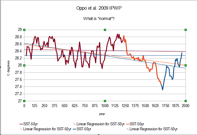
This is the Oppo et al. 2009 recon of the IPWP that I use very often because it correlates extremely well with local temperatures combined with the lower resolution Mohtadi 2010 recon of the same region.  They overlap from 0AD to 1950, but there is very little correlation.  Assuming both authors knew what they were doing, there must be an issue with the natural smoothing and/or dating.  Since both are in C degrees there would be about +/- 1 C uncertainty and up to around +/-300 years dating issues.  If I wiggle and jiggle to get a "better" fit, who knows if it is really better?  If I base my uncertainty estimate on the lower frequency recon of unknown natural smoothing, I basically has nice looking crap.  So instead I will work under the assumption that the original authors knew what they were doing and just go with the flow, keeping in mind that the original recon uncertainty has to be included in the end.

With most of the reconstructions that ended prior to 1800 "capped" with shorter duration reconstructions from the same area, often by the same authors, things start looking a bit more interesting.

Instead of a rapid peak early and steady decline, there is more of a half sine wave pattern that looks like precessional cycle solar peaking around 4000 BC then starting a gradual decline.  Some of the abrupt changes, though not huge amplitude changes in the tropics, appear around where they were when I was in school.  There is a distinct Medieval Warmer Period and an obvious Little Ice Age,  I am kind of surprised the original authors of the studies have left the big media reconstructions to the newbies instead of doing it themselves.

I have updated the references and noticed one blemish, Rühlemann et al. 1999, uses an Alkenones proxy with the UK'37 calibration.  Some of the "caps" are corals since there was not that many to chose from.  Since the corals are high resolution, I had to smooth some to decade bins to work in the spreadsheet.  I am sure I have missed a reference here or there, so I will keep looking for them any any spreadsheet miscues that may remain.  Stay tuned.

And

Since there is a revised version here is how it compares to tropical temperatures.  I used the actual temperatures with two scales to show the offset.  The recon and observations are about 0.4 C different and of course the recon is over smoothed compared to the decade smoothed observation.  Still a mini-me hockey stick at the splice but not as bad as most reconstructions.

references: No: Author

31 Kubota et al., 2010 (32)
36 Lea et al., 2003 (36)
38 Levi et al., 2007 (39)
40 Linsley et al., 2010 (40)
5 Benway et al.,2006 (9)
41 Linsley et al., 2011 (40)
45 Mohtadi et al., 2010 (43)
60 Steinke et al., 2008 (56)
62 Stott et al., 2007 (58)
63 Stott et al., 2007 (58)
64 Sun et al., 2005 (59)
69 Weldeab et al., 2007 (65)
70 Weldeab et al., 2006 (66)
71 Weldeab et al., 2005 (67)
72 Xu et al., 2008 (68)
73 Ziegler et al., 2008 (69)

Not in the original Marcott.
10(1) with Oppo et al. 2009
36(1) with Black et al. 2007
38(1) with Newton et al. 2006
74 Rühlemann et al. 1999
75(1)Lea, D.W., et al., 2003, with Goni, M.A.; Thunell, R.C.; Woodwort, M.P; Mueller-Karger, F.E. 2006

Why is Volcanic Forcing so Hard to Figure Out?

I have a few posts on volcanic forcing and it is very difficult to nail down what is due to what because Solar and Volcanic tend to provide mixed signals.  As far as Global Mean Surface Temperatures go, there is a short term impact some of the time that is easy to "see" but at times volcanic response tends to lead volcanic forcing which you know just cannot be true.  The problem is multifaceted.

First, there are internal ocean pseudo oscillations that are amplified in the NH and muted in the SH.  The SH really doesn't have any room on the down side to have much easy to spot volcanic response and thanks to the thermal isolation of the Antarctic, not much of an upside.  There is a response, just temperature anomaly doesn't do it justice.

However, if you normalize the anomalies by dividing by the standard deviation you can "see" that both higher latitudes, above 40 degrees and the bulk of the oceans 40S-40N have similar responses.  Since the NH has land mass choking the pole ward flow, it has a larger fluctuation, but about the same longer term trend.  Temperature in this case, especially anomaly based on "surface" temperatures doesn't accurately represent energy change.  This gets back to Zeroth Law requirements that the "system" a fair size planet, should be somewhat in equilibrium.  A simple way to see that is a 10 degree swing in polar winter temperatures would only represent about a third of the same swing in the bulk of the oceans.  Around 40 degrees to the poles, the surface has more energy advected from the bulk than provided by solar.  Since advected energy is as or more important than solar, volcanic forcing reducing solar irradiance has less impact.

Second, due to Coriolis effect and differences in land mass, you will have ocean oscillations.  I have previously mentioned that there are three major thermal basins, North Atlantic, North Pacific and Southern Hemisphere with ratios of roughly 1:2:4 which can produce a fairly complex coupled harmonic oscillation.  Since sea ice extent would vary the amplitude, especially in the NH due to land amplification of advected energy, you can just about drive yourself nuts trying to figure out cycles.  Yes, I know that ocean oscillations are a part of both of these reasons.  That is because they influence surface temperature both ways since in addition to providing energy that energy drives precipitation that can produce snow that can reverse the "surface" temperature trend.  In the first case, advected energy offset volcanic forcing and in this case, advected energy causing increase snowfall can enhance volcanic forcing.

To illustrate, this chart compares the Northern Hemisphere and northern high latitude temperature reconstruction by Kobashi et al. with the Indo-Pacific Warm Pool reconstruction by Oppo et al. that I use frequently.  While I cannot vouch for the accuracy of the reconstructions, they should reasonably reflect the general goings on.  The Kobashi reconstruction doesn't have a pronounce Medieval Warm Period since that is more a land based phenomenon, think less glacial expanse, and a less obvious but longer Little Ice Age since land based ice doesn't have much impact on ocean currents other than more sea ice/ice melt can cause impact the THC.  Solar and Volcanic impact on the ocean heat capacity would be a slow process requiring up to 300 year per degree with an average forcing of around 1 to 2 Watts per meter squared.  Impacts felt in the SH may take 30 to 100 years to migrate back to the other hemisphere producing those delightful pseudo oscillations we have all grown to love.  So "natural" variability can cause more "natural" variability since the original forcing can't be sorted out.

In the NH which is more greatly influenced by the oscillations, volcanic forcing on an upswing might have no discernible impact while on the downswing it might have a larger than expected impact.  Add to that potential impacts of volcanic ash on snow melt which would be affected by the the time of year and general atmospheric circulation trends and you have some serious job security if your employer has the patience.

Finally, the southern hemisphere temperature records generally suck big time.  That is simply because the winds and temperatures that work so well isolating the Antarctic  are not all that hospitable for folks that might want to record temperatures.  That means that early 20th century correlations are not reliable.  So there might have been more out of phase situations, the hemispheric "seesaw" effect, that would help determine actual "cause" of some of the fluctuations.

So what does this all mean?  Glacials and interglacials are due to glaciers, ice on land.  They are the number one climate driver so when there is a lot, the climate is more sensitive to things that melt ice and when there isn't much, climate is less sensitive in general.  Since evidence suggests that more ice is more common you can have a lot of climate change without much ocean energy change.  If you want to reconstruct "surface" temperature you need to reconstruct glacial extent.  If you want to reconstruct ocean temperatures, stick to the bulk of the oceans especially the tropics.  Since the Indo-Pacific Warm Pool has lower THC through flow, it would be your best spot for estimating the energy changes in the "global" oceans.

That said, the average temperature of the oceans is about 4 C degrees which happens to be about the "ideal" black body temperature of a rock in space located about Earth's distance from our sun.  Based on that temperature, "Sensitivity" to a doubling of CO2 would be about 0.8 C "all things remaining equal".  4 C by the way is roughly an ideal black body energy of 334.5 Wm-2 which is roughly equal to the best estimates of down welling longwave radiation and since Stefan-Boltzmann included that ~0.926 fudge factor, "normal" DWLR could be between 334.5 and about 360 Wm-2.

If the Oppo et al. 2009 reconstruction is reasonably accurate, then Earth's climate is about "normal" for the past 2000 years, unless you think the Little Ice Age should be "normal".  In any case, things should start slowing down now that climate is closer to the back half of the Holocene mean.

Based on comparing the NODC Ocean Heat/Temperature data, the Oppo et al. 2009 IPWP trend from ~1700 is very close to the projected trend in upper ocean (0-700 meter) average vertical temperature anomaly.  Also while I took some liberties "fitting" lag response times, the combination of solar and volcanic forcing estimated by Cowley et al and Stienhilbert et al.  (Sol y Vol) do correlate reasonably well with the Oppo et al. reconstruction.

To conclude, trying to determine "global" changes in average SST using higher latitude data tends to remove information if the hemispheric "seesaw" is not properly considered and logically the majority of ocean heat should be better represented by the bulk of the oceans of which the Indo-Pacific Warm Pool is a good representation.  To say that there is no evidence of long term persistence/memory in the vast oceans is a bit comical.  

Cowtan and Way Make it to Climate Explorer

Since Lewis and Curry 2014 was published the fans of Cowtan and Way's satellite kriging revision to the Hadley Centers HADCRUT4.something is constantly mentioned as a L&C spoiler.  C&W does run warmer than the older HADCRUT4.somethingless.  I haven't used much of the C&W new and improved version since I like to check regions using the Climate Explorer mask capability.  Well, now C&W are on Climate Explorer.

This is one of my first looks at any data set, tropics, extended slightly to 30S-30N and the extratropics, 30 to 90.  As expected, the majority of the world is consistently warming as would be expected recovering from a period former known as the Little Ice Age and the Northern Extratropical region is warming more because that would be where ice during the period formerly known as the Little Ice Age would have been stored.  Ice/snow is a major feedback and is influences by temperature and dirtiness, albedo.  Industry, wild fires, wind blown erosion, volcanic ash, earthquakes and just about anything that disturbs the pristine whiteness of glaciers and snow fields would impact the stability of the glaciers and snow fields.  So in my opinion, the Rest of the World is a better baseline for "global" warming than the Northern Extratropical region if you want to try and attribute things to CO2, Volcanic sulfates or clouds.  Not that the Northern Extratropical aren't important, but you can see they are noisy as all hell.

Climate Explorer also allows you to use nation masks like the one above for New Zealand.  New Zealand skeptics are quite a bit miffed by the amount of adjustments used by national weather services to create the scary warming trend.  New Zealand is a large island and as such would have a maritime climate.  Since Cowtan and Way krige using satellite data which is heavily influenced by ocean temperatures, the C&W version of New Zealand looks a lot more like the skeptical Kiwis would expect.  I use three tiered 27 month smoothing and left the first two stages in so you can see how smoothing impacts the Warmest Year Evah.  The default baseline for Climate Explorer is 1980 to 2010, the satellite era which would also have an impact on Warmest Year Evah, but not the general trend.  This is a reminder that "Global" temperature reconstructions really should not be used for "local" temperature references since the interpolation, standard or krige, smears area temperatures, good for "Global" stuff but not so good for local forecasting.

 So there is a brief intro to HADCRUT4.something with new and improved smearing.  Not meaning to be a cut down of C&W, it serves a purpose, but increase smearing reduces the relationship between temperature and the energy it is supposed to represent.  Now if C&W had the "skepticism" required they would compile a "Global" energy anomaly reconstruction which would illustrate just how much error using temperature anomaly for temperature ranges from -80C to 50C can produce.  Then they would focus on the "other" forces that effect climate rather than just the CO2 done it all meme.  Since Way is Inuit, I am sure he knows about yellow snow and the variety of other than pristine white varieties.  It would be nice to see him focusing on the whole picture instead of trying to be a good CO2 band member.

Dirty Greenland Glacier courtesy NOAA

Why Pi?

When I mention that the subsurface temperature tends to the energy equivalent of TSI/Pi(), eyes roll.  I use it as a convenient approximation.  If I were to get into more detail, I would use the integrated incident irradiation  which would consider the azimuth of the sun by latitude and time of day with a day isolation factor that included seasonal variations.  Since I am more concerned with the ocean subsurface energy, I would also have to consider land mass and sea ice.

I find it easy to just assume that liquid ocean is most likely between 65S and 65N, then Io*Cos(theta) from -65 to 65 would be about 450 Wm-2 average while TSI/Pi() would be about 430 Wm-2 excluding the land mass.  Those would be average insolation values for the day time portion of a rotation.  If the insulation were close to perfect, these would be the more likely values of the subsurface energy actually stored.

Another reason I like this approximation is that if the oceans were never frozen at the poles, the angle of incidence over 65 degree would mean close to 100% reflection off a liquid surface anyway.  The only energy that would likely penetrate to the subsurface directly would be between roughly 65S and 65N except for a month or so in northern hemisphere summer.  It is a lot easier to say the subsurface energy will tend toward TSI/Pi(), than to carry out a lot of calculations which are about useless without knowing the actual cloud albedo at each and every location on Earth.  Roughly though, if you consider a noon band with a zero tilt and the average 1361 Wm-2 TSI, from 65S-65N the insulation could be as high as 910 Wm-2 versus 665 Wm-2 for 90S-90N for the oceans.  That should give you an idea of the difference between subsurface and surface solar forcing using average ocean land distribution.  There are of course central Atlantic and Pacific noon bands with nearly zero land mass between 65S and 65N that can allow much more rapid subsurface energy uptake.  So until I either take the time or determine a need for a more accurate estimate, TSI/Pi() is convenient.

Purist won't like that, but hey.

There are quite a few things that can bung up that estimate.  One is how well the subsurface energy is transferred pole ward.  If the transfer is slow, like before the Panama closure, the equatorial temperatures would tend higher which could increase the average or the Drake Passage could open which would decrease the average.  When the average changes the cloud cover percentage and extent would change making the puzzle a bit more challenging.  With a baseline, "surface tends tend toward TSI/Pi()", you can at least estimate the impact of changes in ocean circulation on average ocean energy.  It is far from perfect, but a convenient approximation.  It is also convenient to assume that albedo is fixed.  Subsurface versus surface energy provides a reasonable explanation why albedo may be some what fixed.

If you have a more elegant estimate, break it out.


Note:  This post is just an explanation in case some wants more detail about the TSI/Pi() approximation.  It may be revised or expanded as required.

Normal?

	TSI	Albedo	Surface	subsurf.	App. Surf.
			TSI/4	TSI*(1-1)/Pi()	TSI*(1-1)/4	Sub-App	Wm-2/K	K/Wm-2
Winter	1410	0.215	4.00	3.14
		Wm-2	352.50	352.32	276.71	75.79
		Eff. K Degrees	280.80	280.76	264.31	16.45	4.61	0.22
Summer	1310	0.215	4.00	3.14
		Wm-2	327.50	327.33	257.09	70.41
		Eff. K Degrees	275.68	275.65	259.49	16.15	4.36	0.23

Based on the Forcing, Feedback, Response and other Mumbo Jumbo post here is a little table for the more realistic conditions on Earth.  All of these are still "ideal" estimates meaning take with salt, but if we didn't have an upper atmosphere reflecting sunlight and molecules getting t-boned by higher energy photons/particles, we might have the actual estimate Total Solar Irradiance (TSI) "felt" at some easily "seen" atmospheric level we will call the Top of Our Atmosphere (TOOA) not to be confused with TOA, another idealized estimate.  The App. Surf. is the Apparent Surface that some space ship tooling around would see.  In order for the Earth to exist when the space ship tourists arrive, the Energy in would need to be pretty close to the energy out.  With any luck the tourists measurements will suck as much as ours and they will say Ein = Eout and not worry about minor uncertainties.

If they arrive in Winter, they might be surprised that our planet is colder than they would expect and if they arrive in Summer they might think Earth is not going to be around much longer because it is over heating.  

You should note that in the chart, albedo is lowered to 0.215 from the conical 0.30.  I did that so the energy calculations for the surface and subsurface would be the same.  That would be an equilibrium and/or steady state condition required by a less than perfect black body with a semi-transparent fluid atmosphere/surface but still homogeneous by design .  In the real world, some portion of the albedo is provided by the cloud surface, some portion is provided by the physical surface and some portion provided by the above the cloud surfaces.  The majority, about 72% is provided by the base clouds, which are...?  That is right sports fans, a response to surface and sub-surface temperature.  

Since Earth has a less than perfectly circular orbit, there is a small difference between Winter and Summer and in the far left column you have a 0.22 and 0.23, K/Wm-2.  That would be the apparent "Sensitivity" in degrees K per Wm-2 observed.  Since the observed energy depends on the atmospheric response required to equalize Tsurface and Tsubsurface, the Ein=Eout requirement is co-dependent on the Esurf=Esubs requirement. 

Earth also has an orbital tilt peculiarity.   That means that TsurfNH and TsurfSH, for the hemispheres, would also need to find a happy place.  This is before considering all the issues with real estate location.  Our Ideal Model of Earth already has a number of co-dependent equilibrium/steady state conditions that must be met or no Earth as we know it would exist.  Most of the flexibility needed to meet the conditions is provided by the rapid climate response cloud team.  

While this isn't all that complex to me, some get confused by more than one equilibrium/steady state requirement and try to simplify (over simplify IMO) to a single requirement.  You need to be extremely careful with the likely long list of simplifying assumptions needed for that degree of reductionism because they are ASSUMPTIONS not facts.  Jumping in to debate issues with overly simplified models is a bit like arguing with a drunk, doesn't do much good.

If you aren't into arguing with drunks, a tad more complex model would include another "surface" located above the normal cloud base in the drier part of the atmosphere.  This would be the surface layer where increased CO2 would play a larger role.  To play with that layer, the Remote Sensing Systems (RSS) Temperature Lower Troposphere (TLT) data which is available in absolute temperature format with masking ability from Climate Explorer can come in handy.  This can provide an approximation of the subsurface for the dry air "surface" portion of our puzzle.

With a rough average of 272 K degrees, about one C below freezing, available "subsurface" energy at a minimum would be 310 Wm-2 and thanks to a very narrow atmospheric window, about 20 Wm-2 of extra energy "MAY" be available at any time if you would like to get more detailed.  Note that my mask is for 65-65 degrees or the portion of the surface that is actually illuminated year around thants to the peculiar axial tilt situation.  At the poles especially during winter, they would be part of the dry "surface" and in the Antarctic most of the area would be "dry" all year.  Trying to lump in these dry surfaces would tend to overly complicate this supposedly simple post on co-dependent thermodynamic states which doesn't "solve" anything, just introduces another way of looking at the same tired old problem.

When you have two or more co-dependent states with different response times, you can expect oscillations or hunting while the states try to find their happy place.  When you have several co-dependent states, you can expect more interesting hunting.  But if you know the preferred state, then you can make some progress without resorting to Chaos Math, which I consider an nice thing.

Forcing, Feedback, Response and other Mumbo Jumbo

Now tell me, which came first,  the chicken or the egg?  Discussions of Forcing and Feedback can be about like that.  When some talk about the greenhouse effect they mention that the "Earth is 33C warmer than it would be if there were no Greenhouse Gases".  I guess they think the egg came first?

With no atmosphere, the Earth would have a "surface temperature" of about 4 C degrees based on TSI/4 or ~1361 Wm-2/2 = 340 Wm-2 which if you assume a very perfect black body, the Stefan-Boltzman Law would give you an effective temperature of about 4 C degrees.  If the Earth were a less than perfect but close black body, the "subsurface temperature" with no atmosphere would be about TSI/Pi=433 Wm-2 which by the S-B law would be a temperature of about 22.5 C degrees.

The subsurface temperature would be due to one and only one radiant surface, the assumed to be ideal surface, that would produce an average of ~4 C degrees.  Instead of an atmosphere insulating the surface, a few meters of assumed uniform soil of some sort provides insulation.  There is a page on Lunarpedia related to lunar temperature you can check if you like.  If the actual absolute "surface" temperature of the Earth is 15C, then Earth's "surface" temperature would fall right in the range of an "ideal" black body surface and subsurface.  If our atmosphere thickens or becomes a better insulator, the temperature would increase to closer to the subsurface 22.5 C and if it thins, closer to the 4 C surface temperature.

No where have I mentioned clouds or CO2 or anything forcing/feedback related.  This is what I consider the egg.  This is why I continually ask for a better definition of the "surface" folks are talking about in reference to Global Warming or the Greenhouse Effect.

The actual Earth doesn't have a uniform "ideal" surface/subsurface it has oceans.  The "average" temperature of the ocean subsurface is about 4 C degrees.  That is likely due to a variety of "lucky breaks".  The first lucky break is water has a weird maximum density at 4 C degrees.  Even though that is for pure water, the salty oceans still are influence by the 4 C density phenomenon and the ~0 to -2C freezing point of the current blend of fresh to salty water.  The second lucky break is that water which is close to an ideal black body provided it isn't frozen or evaporated, would tend toward the ideal black body temperature related to TSI/Pi.    That's right sports fans, if there were no clouds the oceans average temperature would be close to 22.5 C degrees.  The third lucky break is that as the briny oceans saturate with salt, the freezing point can drop to about -18 C degrees.

If you have ever looked into solar ponds, a heavy brine subsurface with a stratified fresh water lens makes one hell of a solar energy collector.  That makes it very difficult for Earth to remain a "snowball" for any length of time as long as there is the sun and salt limits in the equatorial oceans.  It also means that there will be considerable water vapor if the oceans are not frozen over.

With warm equatorial oceans there will be water vapor in the atmosphere.  Water vapor is also a greenhouse gas, but it is limited to a more narrow temperature range of roughly -43 C in a "normal" atmosphere but in a very clean atmosphere with very few cloud condensation nuclei (CCN), the limit could be as low as -100 C degrees depending on the overall concentration.  How much impact water vapor all alone would have on "surface" temperature I have no clue.  The atmosphere of the Earth also contains oxygen which in strong solar irradiation reacts to form ozone mainly near the equator.  I have seen estimates that tropical ozone and water vapor advected towards the poles increase the temperature of the highest latitudes by about 50 degrees in a very critical region.  So we have two greenhouse gases, ozone and water vapor that exist due to solar irradiance, atmospheric composition and oceans that are responses to the circumstances, "lucky breaks", that are not easily classified as forcing or feedback.  Changes in water vapor and ozone can be feedback or forcing or more realistically responses to general system conditions.  You would have to define "normal" in order to pigeonhole the changes.

With warm oceans and some CCN, there would be clouds which tend to reflect solar irradiance.   That in my opinion is a response which can become a forcing or feedback depending our your perspective i.e. frame of reference.   Since the subsurface depends on the solar insulation at the surface, clouds a few kilometers above the surface would tend to reduce the solar impact.   Remember that if the actual albedo of  the ocean area is 0.23, then the subsurface temperature would be 4C using the (1-a)*TSI/Pi approximation.  Try that on your own just for kicks.

This is were climate science in its "Global Warming" mode went wrong in my opinion, they assumed a normal instead of considering a range of normal that would be related to the surfaces selected as references.

As it is, additional CO2 would increase the atmospheric insulation potential and the impact would always depend on the current conditions.  The largest of the current conditions would be the average temperature of the oceans which have that tendency toward a 4 C average as a relatively clear liquid subsurface.

So now go figure out what "discrepancy" there might be in "surface" temperature.

More Missing Heat Stuff - Southern Hemisphere

Every since the ARGO system has been in place the missing heat disappearing into the deep oceans has cropped up.  The ocean heat content change is one of the most questionable of all climate data sets.  The huge change in energy in 10^22 Joules is based on sparse measurements of vertical temperature, pressure and salinity over several various data acquisition types.  Pretty much a hodge podge of methods spliced together with some serious statistical approaches.

I have said before that I am pretty impressed that the data looks as good as it does, but I am not all that convinced that the error ranges are all that accurate.  Because of the "almost unbelievable" certainty, any adjustments will likely be small in order to not embarrass previous guestimators.  

This chart, pardon the mess and misspellings, show the southern hemisphere Vertical Temperature Anomaly (VTA) for the 0-700 meter and 0-2000 meter ranges with the southern hemisphere sea surface temperature from -60 to the equator.  Notice how the SST and the VAT are almost mirror images across a trend line.

If I invert the SST across it's trend line you can see how well they match up.  When the SST cools or stays neutral, the deeper ocean warm a little.  Nothing particularly shocking about that, changing the surface winds and currents changes the efficiency of the mechanical mixing efficiency some like to call eddy diffusion rate so for this chart about 0.6 C of surface temperature increase produce about 0.14 C of warming in the 0-700 meter ocean layer.  Should all things remain equal we might expect about 25% of the warming to be sucked up by the oceans.

If I compare to the 0-2000 VAT my correlation isn't quite as good.  That might be the way things are or then again since ARGO only started around 2003, it might be due to a bit of wicked instrumentation change force fitting.  That would be a fairly steep leap in 0-2000 meter temperature between 2001 and 2013 wouldn't it?  Almost unbelievable.  Since the energy to warm the deeper oceans had to come from somewhere, I would think there would be a better fit.  Perhaps not, but one, 0-700 meters appears to make more sense than the other 0-2000 meters and there is a reason to question the 0-2000 meter data, very little existed prior to 2003.  As they say, if sounds too good to be true it probably is.

What is a Hoax?

The more devote of the Climate Change believers despise the "skeptics" calling Global Warming a hoax.  Remember Global Warming was the first name for the "crisis" which then morphed into Climate Change and then Climate Disruption.  Why the name changes?

The Penn and Teller DiHydrogen Monoxide hoax is a good example of a hoax than deceives with the truth.  It is a play on ignorance and faith.  "Believers" take the truth and let their imagination run wild.  A hoax doesn't require a hoaxer or someone planning the hoax.  People can deceive themselves with out any assistance at all.

What Really Happened, is a web page that has a fairly extensive list of things claimed to be caused by global warming.  The beauty of a well planned hoax is to let the audience do it to themselves, like the Penn and Teller skit.  Once a seed is planted,  observers should be able to have a great many laughs as they watch players convince themselves and others of a relationship that continues to grow more and more unbelievable.  At some point, MOST should catch on an realize the humor.  Some never will though.  That is the sad reality, a good joke is wasted on many.

Global warming, at least the Catastrophic end of the world version, has become a joke and we are now stuck watching the least sharp tacks in the box flail around.  Not fun.  A joke needs to be appreciated by as many as possible.

What is the "Right" Solar Reconstruction?

I have played around with Solar a few times and found some interesting things but there is nothing very persuasive considering no one is in any kind of agreement how solar really should be handled.  My biggest issue is that solar has its strongest longer term impact in the near tropicial oceans, rough 40S to 40N and short term impact in the NH land areas from around 25N to 60N.  There is also a "year" issue.  Since a Solar year is not the same as an Earth year and months are a pretty Earth only related time frame, you get a better correlation between solar and the tropical ENSO region using a 27 month lag which would likely be better with some fraction of a month.  Using daily data is a huge issue for my laptop, but would be the best way to go with things.  Anytime you try to determine correlations between averaged data sets there will always be some issue that could be extremely critical if you are talking with the serious statistical guys.

Solar "TSI" is a bit of an issue also.  You really should use spectral intensities which once you add that to daily or some number of hour records gets to be a huge database for the laptop tinkerer.  On top of that, solar reconstructions require different scaling factors due to issue with different data types and lower atmosphere solar has a lot of background "noise" or maybe signal that could be related to atmospheric optical depth.  It is one big ass can of worms.

Still, it is hard to avoid tinkering with solar correlations despite the issues.  I did the above chart just for grins.  The maximum correlation I could find between solar "TSI" anomaly and the "tropical" ocean SST (30S-30N is a bit more than just tropical) is 56% which is nothing to write home about.  It is probably just enough to inspire more looking, but not enough to convince anyone of anything.

The 4 year lag used to tweak the correlation is about half of the settling time Steve Schwartz estimated for the bulk ocean layer.  To me that would suggest that there is a fast response plus a lagged response of about equal intensity.  I have combined different TSI lags in the past and can get just about any correlation I like up to about 87% or so depending on which surface temperature data set and area I pick.  That gives me way too many degrees of freedom to trust.  All is not lost though.

Since there are quite a few published papers noting links between ENSO and reconstructed TSI, the average tinkering Joe cannot be classified a complete whack job because he has "professional" company.  The trick is coming up with a compelling rationalization .. er explanation, of why you used what in your "analysis".

 I am sticking to my multiple lag theory because ocean heat transport would support a number of lags and sub surface insolation which highlights the tropicalesque ocean influence on long term climate.  So instead of using Land and Ocean temperature data, ocean only should be a focus with a possible Ocean plus 8 year averaged Land hybrid temperature data set.  That would basically incorporate the ocean settling lag making the "global" temperature series a bit less noisy without having to cherry pick an averaging period.

This is what MAY be my choice of data sets for comparison to solar.  Note that I used a Pre-CO2 baseline, since ACO2 supposedly didn't kick in until ~1950.  I used two different scales just for this comparison to show that my cherry picked, er selected regions tend to agree.  I used the GISS 1250 km interpolated data though the 250km data would normally be my choice.  Since the highest latitudes aren't included there isn't much difference.  This chart is just to show that using just the 30S-30N tropical ocean, I am not losing touch with global temperatures as much as some might think.  The tropical ocean would be the major source of global energy after all.

There is a good chance this is a far as this will ever go unless I bite the bullet and download daily data.  In case you are wondering, the excluded high latitudes contribute about 18.5Wm-2 (north) and 13 Wm-2 (south) to the "global" effective energy.  The rough average effective energy of the 60S-60N region is ~410 Wm-2 so the exclusion would add about 7.5% to the energy uncertainty versus about 12.5% to the temperature anomaly uncertainty.  One of my pet peeves about manufacturing temperature data in the polar regions is that it artificially doubles the impact in some cases