RMS versus Average - the Radiant Shell Game

This is the problem.  Assuming "average" instead of RMS you have figure (a)  With RMS you have figure (b) as a peak and (a) as zero.  As the total heat content of the surface with average energy value (a) increases, the range of (b) minus (a) changes.  For a "ballpark" estimate, (a) is fine, but since the variation from (a) to (b) can be 17 Wm-2 equivalent or more compared to a total CO2 forcing of 4Wm-2, the "ballpark" estimate is not adequate.

The link to the article containing that graphic is, Science Focus: Sea Surface Temperature Measurements MODIS and AIRS Instruments Onboard of Aqua Satellite

If you are looking for "average" and get something else, you might start blaming the satellite guys.  So let me try to compare the "average" and RMS values of the energy applied to the "surface" again.

Surface is in quotes because there are various surfaces in a complex system.  The ocean atmosphere interface or boundary layer is one of the more important surfaces.  The actual solar energy that can reach this surface varies with cloud cover, season, time of day, and there are longer term "minor" solar cycle variations.  The energy provided is always positive, ranging from zero to roughly 1410 Wm-2.

A simple average for a sphere with 1410 Wm-2 available would 1410/2=705 Wm-2 for the active or day face and 705/3=352.5 Wm-2 for the diurnal average.  An RMS estimate based on the sinusoidal shape of the applied energy would 1410/1.414=997 Wm-2 and due to spherical shape 997/1.414=705.  Since there is not abrupt fall to zero with day to night transition, for diurnal change the RMS value would be 705/1.414=498 Wm-2.  Cloud cover is generally non-stationary, so local variations change with some unknowable time period, amounting to roughly a pulsing energy wave shape with some average duty cycle.  Since most tropical clouds form after peak solar from energy gained up to peak solar, the cloud cover effectively shifts the "surface" upwards.

If you neglect the clouds for the moment, the 498Wm-2 is the RMS energy at some "surface".  As a radiant "shell" that surface would emit energy up and down, producing 259 Wm-2 up and 259 Wm-2 down.  Then the RMS value would be equal to the "Average" value, but that requires an ideal "surface" with precise depth and negligible thermal mass.  To maintain the energy in that radiant "shell" there must be 259Wm-2 provided constantly from some source, i.e. an ideal black body.

Clouds plus changes in atmospheric density and composition would vary the depth and distribution of the "shell", but the "shell" energy is solely dependent on the two black body sources, the Sun and the thermal mass of the core.  Since the core must store energy gained from the Sun, the nocturnal energy available depends on the core's ability to transfer energy to the radiant "shell".

I am going to stop here to let everyone ponder this concept with a little food for thought,
E=Eo*e^(-t/RC),  what is "t" for a planet?

The RMS Challenge

My why RMS has been challenged.  Hey, I can be wrong, so let's take another look.  The challenger said that solar is a half rectified sine wave.  That is close enough, though the last time I looked, the sun transformer did not have a center tap.  The solar input is actually a full peak to peak sine wave,  There is no negative energy assumed for this example.

 Well a half rectified sine wave has a full half cycle of zero voltage.  We have that with the sun.  Then next half cycle has full peak to peak voltage instead of just peak.  It is assumed to be just peak because the surface is spherical, but that surface also doesn't get negative energy.  The RMS value for that cycle would be peak-peak/(2)^.5 or 0.707 times Peak-Peak.  So what's the difference?

Pretty much that.  The half wave rectification would have a full 50% duty cycle.  The full wave is basically just a floating sine wave so the RMS value would be Peak/1.414.  Since the Peak is what would be the Peak to Peak for a normal alternating current wave form, you have a larger amount of energy that is obtainable.  With the partial wave on direct current, you would have an RMS value equal to the pulsing portion of the wave form.  As the DC component increases, the pulsing portion would have less impact.

There are always more ways than one to skin a catfish, so the climate science method of total solar energy divided by four works, but only if you consider the thermal capacity of the system.  That would be the DC portion.

I only bring this up, well, because of the challenge, and because the solar cycle has inconsistent periods which would be like pulse width modulation.  Depending on the internal rate of energy transfer, shorter solar periods could partially synchronize with the internal cycles creating a larger "DC"impact.  Since the oceans have the potential for extremely long lag times, longer term solar modulation could also synchronize.  Not considering the RMS values of both the input energy and the internal energy would lead to potentially large mistakes.

Update:  As a little ps, if there is no thermal capacity, then the RMS values in the latitudinal and longitudinal direction would multiply to 0.5 which would produce the TSI/4 estimate for "average" insolation.  Since the equatorial band would store energy, achieving the TSI/4 estimate would require perfect radiant heat loss.  I am pretty sure nothing is perfect, so RMS should be considered.

Energy versus Anomaly

Since the BEST project is adding a new combined land and ocean product to their list, I am not going to try to beat them to the punch.  I will provide a little preview of what their new product may reveal.

Since the cumulative impact of the Pacific Decadal Oscillation is a topic on one of the blogs and the mystery of the 1910 to 1940 "natural" peak as well, I thought I would try to combine both.  The BEST land data provides Tmax and Tmin temperature series with estimates of absolute temperature.  Using the Stefan-Boltzmann relationship, I converted the Diurnal Temperature Range (DTR) to Diurnal Flux Change (DFC) for this chart.  That is just the energy anomaly associated with DTR.  A 21 year trailing average was used to "simulate" accumulation with respect to the ~21 year Hale solar cycle.  Different averaging periods would "smear" the peaks if longer, producing a neat 1910 to 1940 peak if that is what you really want.  Since Washington State and Canada were used, there would likely be some PDO influence, but since the AMO or Atlantic Multidecadal Oscillation is just across the way, the differential between the two would likely be a stronger influence than either independently.

If the new BEST product produces reasonable absolute temperature estimates, then it could produce reasonable absolute energy estimates.  The following the energy through the system would be much simpler than it is now.  It is after all the energy that creates the temperature anomaly squiggles, so some bright young scientist may soon be new Sultan of Schwung using BEST products.

Update:

The frustrating part of this whole puzzle is the Telescope Jockey "averaging" simplifications.  In Astrophysics, if you can estimate the temperature or energy of a body in space to +/- 20 Wm-2, you are kicking Astrophysics butt.  We are not on a distant body floating in space though.  We are on our home planet with much more than just radiant physics estimates to draw upon.

Here, we have a pseudo-cyclic power supply, the Sun, and asymmetrical hemispheres with different thermal capacities and time constants.  That is why RMS values of energy should be used and more model "boxes" included depending on how accurate one would like to be.  There are layers of complexity to be considered.

Since there are Two Greenhouses with several spaces in each, radiant assumptions on a short time scales, less than a few thousand years, just ain't going to cut it.

Layers of Complexity

When I first started playing with this climate puzzle I mentioned to a PhD in Thermodynamics that using a true "surface" frame of reference, the problem was simplified.  The PhD in Thermodynamics promptly told me that I wasn't using "frame of reference" correctly.  Not that I had selected a poor frame of reference, but that frame of reference just didn't matter.  My how thermodynamics have progressed since I was in college.

The CO2 portion of climate change should, with the current levels of CO2 produce between 0.2 and 1.2  C degrees of warming based on a 1900 to 1950 baseline.  Since 1900, the warming has been roughly 0.7 C degrees with some portion of that warming likely not directly related to CO2 impact.  Since there is an environmental lapse rate that varies with altitude and some degree of internal variability, selecting a frame of reference that is not very specific would likely not produce anywhere near the accuracy required to tease out individual impacts.  That is my opinion based on limited pre-turn of the century Thermodynamics.  If you pick the wrong layers, you get noise.

Since I didn't keep up with all the changes, I tend to look at things as parts instead of a whole until I figure out what makes the whole thing tick.  Using the HADCRU SST and Tropical Surface Air Temperature data I made the above chart.  I used a 12 year sequential standard deviation because it is in the ball park of the 11 year solar cycle and I didn't want to get into half years.  Compring the data, the NH doesn't play the same as the SH.  Since the HADSST2 data set doesn't include a tropical dataset that is easily accessible, I used the new HADCRU4 tropics as a reference.  The next chart is simply subtracting the NH and SH from my Tropics reference.

The blue and orange curves are that subtraction for the tropics reference.  I added the Solar yellow curve based on the Svalgaard TSI reconstruction using an 11 year sequential standard deviation since I still don't want to get into half years.  I could have done things differently, but for an illustration is doesn't really matter.

To help show what I am trying to explain I have added a linear approximation of the Solar reconstruction with two regions defined, Transition Phase and Control Phase.  Without trying for much detail, from roughly 1900 to 1960, Solar energy could be absorbed more efficiently as the systems transitioned into a new state or phase.  That is roughly a 60 year period that may or may not be cyclic. Once the Control Phase is reached, the systems respond differently to forcing.  What may have the greatest impact in the transition phase would not have the same impact in the control phase.  If the oceans had lower heat content prior to the transition phase, then the control phase could be based on a new ocean heat content limit.

That limit could be based on total ocean heat content or relative ocean heat content.  Since the NH responded differently during the transition phase than the SH, internal transfer of energy to the two hemispheres is a likely contributor to the change.  If that is the case, then in the control phase, less energy would be used to equalize the hemispheres and there would be more energy loss to the atmosphere on its way to space.  Since the NH was gaining more of the transition energy, it would have a greater atmospheric impact during the control phase.  Why?

In the NH there is more land mass and less ocean mass.  The average altitude of the air over the NH land mass is around 2000 meters in altitude which would have roughly 20% of the density of sea level air.  It take less energy to warm a lower density volume than a higher density volume.  The impact of ocean hemispheric equalization would be amplified.  The land mass also has a lower thermal capacity than the ocean mass.  Since land mass can store less energy than ocean mass, the NH response would be different than the SH response during any phase.  With the NH oceans "charged" and the lower land and air thermal capacity limiting the storage potential, more energy would be lost to space during the control phase in the northern hemisphere than in the southern hemisphere.  This may or may not trigger another phase change, depending on the energy supplied to the oceans.

There is no magic involved, the energy storage efficiency just changes.  There are dozens of different influences than might be negligible in the transition phase that would not be negligible in the control phase.  Since the internal energy transfer in all phases depends on both the ocean greenhouse effect and the atmospheric greenhouse effect, you have to consider both.  There is no single, linear climate sensitivity.

Battle of the Thermal Equators

Averaging a world of energy flow is not something I find all that interesting.  There is a cause for the "wiggles" and since there is no general agreement on the impact of the natural wiggles over any time period, understanding the wiggles requires more than simple averaging.

The Earth has a power input from the Sun that is centered in the southern hemisphere during this phase of the precessional and obliquity cycles.  The solar input is not uniformly distributed, so there is not rational reason to assume that it is other than lack of curiosity.  Since I don't have all the software set up to accurately determine the true "solar" thermal equator, I can use the GISS LOTI 24S to 44S temperatures to approximate the impact of variation in solar forcing.  Since the sun has roughly 11 year cycles, I will use an 11 year sequential standard deviation to simulate an RMS input "shape".

With the internal energy transfer from this solar "thermal equator" to the atmospheric "thermal equator" likely to require some time, I can compare the GISS LOTI 24N to equator to the solar "thermal equator" to estimate a delay in the energy transfer.

The blue curve is the difference between the solar equator and the atmospheric equator.  Just for fun, I added the Svalgaard Total Solar Insolation (TSI) reconstruction using the same 11 year standard deviation to simulate an RMS "shape" of the input power.  There is a lag of 5 years required to match these two curves.  Is the match perfect?  No, it would be silly to think that there would be a perfect match, but there does appear to be some significant correlation.  Since the solar thermal equator is south of the atmospheric thermal equator, there is actually even a reason for there to be a correlation.

Shocking!

Why Root Mean Squared?

 If you live in the United States and have a toaster, it is like rated for 120 volts and 15 amps or less.  Those values are RMS or Root Mean Squared values.  The actual alternating current provided by the wall receptacle that you plug the toaster into is supposed to be 340 Volts peak to peak and the breaker that serves the receptacle is likely rated for 20 or 15 amperes.  To figure out RMS, you have to consider the shape of the wave form providing the energy.

For just the basics, Wikipedia has a fair page on the subject.  Since the toaster is AC with a Peak to Peak of 340 Volts, the sine wave formula applies, RMS=0.707*a, where the 0.707 is the square root of two and a is amplitude or peak value, not the peak to peak value.  So the toaster gets 0.707*170=120.19 VAC, or just plain 120 or even 110 volts depending on the leg of the transformer your toaster's breaker is connected to at the panel.  What's is a few volts among friends.

So what has this got to do with climate science?  Probably a lot more than many think.

For the toaster, the RMS value is great because the AC voltage in goes positive and negative.  Since the toaster is likely grounded or at least insulated, in the middle of the sine wave current is zero.  It draws current on the positive and negative parts of the sine wave.   The current then would be in phase with the voltage.  Let's say that we have a floating neutral.  That would be where zero is not in the center of the sine wave but shifted up or down, the neutral of the transform is not grounded.  In this case, since we really don't know what the peak is, 0.707*340=240 volts might be the voltage applied to the toaster.    Since the toaster is a resistive load, now the current may be out of phase with the voltage, how much we don't know without checking things out.  Got to know your reference or ground state.

Since the Earth rotates, the energy provided by the sun is a sine wave effectively with a peak to peak value of 1360 Wm-2.  0.707*1360=961 Wm-2 would be the RMS value of the energy applied if the Earth were a flat disc.  Since Earth is spherical, that energy is at a peak near the equator and near zero at the poles so the cosine distribution would be 0.707*961=679 Wm-2.  This is twice the applied energy generally considered with the  TSI/4 average used in climate science.  This doesn't mean that climate science is wrong, just that there are other ways of looking at things.

The 679 Wm-2 is just the RMS value for the day surface.  Related to a fixed ground level of zero, the mean would be 1/2 or 339.5 Wm-2 or about the same as the 340 generally used.  But if the "neutral" is floating, i.e. there is something other than zero as a reference, the actually available energy would be higher.  One possible source of a floating "neutral" is the Greenhouse Effect.  Since it takes time for the night side to decay to "zero" or "neutral", Greenhouse Gases as well as other atmospheric effects would increase the delay.  Since there are two greenhouse effects in my opinion, I want to look at the other first.

The oceans also have their own delays in heat loss.  That residual energy left before the next day dawns, would effectively cause the floating "neutral".  Since the thermal mass of the oceans is much greater than the atmospheric, this residual energy would be the "source" of the atmospheric portion of the Greenhouse effect.  This is not disputed, but methods used to isolate the total impact of the atmospheric portion tend to assume away to impact of ocean thermal inertia or the lag required for the oceans to decay to a "zero" energy value.

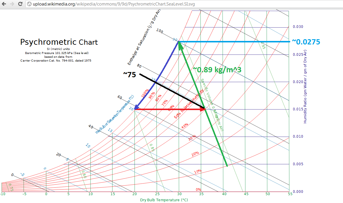
The heat of fusion of water is just one of the inertia lags.  The latent heat of fusion, ~334 Joules per gram of water and the "energy" of fusion of 316 Wm-2 down to ~307 Wm-2, could provide a total energy of up to 334 + 316 = 650 Wm-2 is the area of surface and volume of ice happen to be equal.  So if the surface water can freeze quickly and deeply, it could release pretty much all or more of the energy gained in the day period, since the difference is only 29 Wm-2 and there are of course other factors.  I am going to use energy values instead of temperature for a reason that will hopefully explain itself later.

The question is how quickly.  For ice to form in fresh water it would first cool the water to maximum density, ~316 Wm-2.  The as the water freezes, releasing the 334 Wm-2 of energy, the density of the ice decreases to approximately 90% of the maximum.  This increasing density first then decrease, produces an counter flow that would delay heat loss.  Since fresh water has a maximum density at 4 C, the whole volume would have to cool before ice began to form.  Since the oceans are a huge volume, the rate of heat transfer would "define" a volume that could freeze.  With salt water, the maximum density is not limited to 316 Wm-2.  It would be limited by the energy and salinity.  The Fahrenheit temperature scale is based on the freezing point of saturated salt water or brine at 0 F and fresh water at 32F.  0F or -17,7 C has an equivalent energy of 241 Wm-2 (255.3K degrees).  Since salt is expelled in the freezing process, ocean water freezing would create a lag or delay from nearly 316 Wm-2 to 241 Wm-2.

Now to hopefully answer that question in the title, because of inertial limits.  In order to reach a perfect peak energy, things have to be perfect, the insulation of the capacitor, zero resistance in the transfer, perfect stability in the applied power.  Our world operates in okay ranges not perfect ranges.

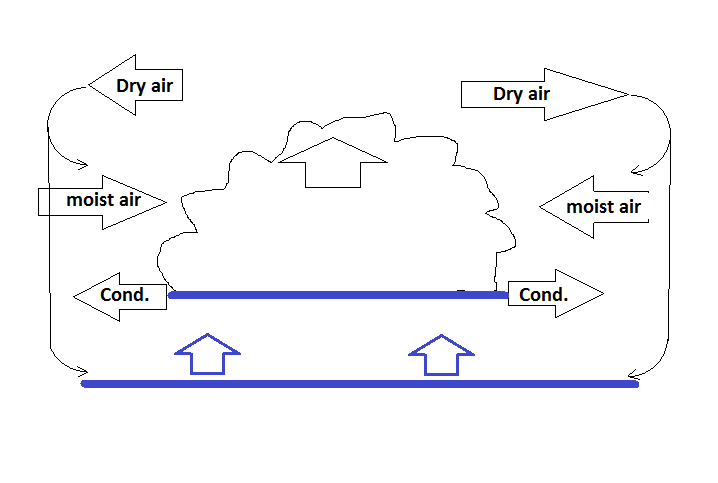
Think of the oceans if we were to turn the sun off.  They would cool fairly rapidly until they reached about 316 Wm-2.  Then they would have to release about twice as much energy to continue cooling, so cooling would slow as they approach this inertia limit.  Since the oceans have salt that would be expelled in the freezing, not all but most, that expelled salt has to diffuse or mix away to allow less saline water to freeze.  That is another inertial limit.  Then once all the oceans have reached approximately 0F or -17.7 C, then the inertial limit is passed and more rapid cooling could begin again since counter flow mixing is no longer required.

It is like charging a battery, lots of current to start decaying to zero at full charge and when you discharge, there always seems to be a little energy left it you let is set a little while, the "floating neutral".  It is all in the mixing.

Back to the Carnot Efficiency with a Little Entropy

One of the bloggers mentioned Carnot Efficiency would be a good way for the climate science gang to validate their estimates.  I have mentioned to him in a post that Carnot Efficiency wouldn't likely be much good since absolute temperatures were not up to snuff.  I have a fairly decent estimate of Tc or the cold sink at 184.5 K degrees +/- a touch.  Th, or the hot source temperature is a lot harder to guestimate.  Since the TOA emissivity is close to 0.61, the efficiency pretty much has to be close to 39%, but I am not sure how much good that would do since before long we will need to add more significant digits.
 
Part of a real cycle though is the Clausius inequality.  There is always going to be some energy that cannot be used and part of that is source temperature changes don't have time to be fully utilized.  Once you get a system in a true steady state with stable source and since, efficiency can improve, like a gas turbine.

Since Earth has a diurnal energy cycle, some portion of that energy will never be utilized.  This brings us back to whether the RMS value of the Ein cycle should be used or the Peak value.  Since the average energy value of the oceans appears to "set" DWLR or lower atmospheric Tmin, it would be more likely the steady state "source" for the atmospheric effect.  Tmax, which is a bit elusive with the SST issues, is little help right now, but Tave, using the Aqua and BEST data should be close to 400 Wm-2 or 17.1 C degrees.  With 400 Wm-2 as Fave, or flux average and 334.5 Wm-2 as Fmin, or really Fconstant, we have about 65Wm-2 of energy flux which is transient or cyclic.  Some portion but not all of that energy would be available to do something.

Using the Carnot Efficiency, (Th-Tc)/Th  With my rough values, (303-184.5)/303=39.1% with Th-Tc= 118.5 K degrees.

I can also consider the ocean efficiency.  Since the ocean sink is much warmer, ~271.25K (-1.9C) with the same source of 303 K, (303-271.25)/303=10.5 percent with Th-Tc=31.35K degrees.  With the ocean "engine" having a lower efficiency, the ~65 Wm-2 would have less chance of providing as much useful whatever.

Making a large assumption, I am going to assume that the ocean can only use 10.5/39.1 or 26% of the transient energy.  That would be 17.4 Wm-2 of possibly usable transient leaving 47.5 Wm-2 as a rough estimate of unusable energy or entropy.  

Whether you followed all that or not, it just means that the ocean "engine" is much less efficient because of the smaller difference in source and sink temperature.  Since it has a lower efficiency and exposed to the same transient energy, it would have higher entropy at the surface.  The atmosphere may make use of more, but with a lower thermal mass, it would be unlikely to retain what it does use.

How this amount of entropy would manifest itself in a open system like Earth climate may not be that difficult to figure out.  The "atmospheric window" energy is the likeliest candidate and these rough numbers are not too far from the measured values.  There is one issue with the "window" energy and that is what surface(s) emit that energy.

It should be reasonable to assume that water, with its larger radiant spectrum releases most of the "window" energy and that since water is in the atmosphere, that both the surface and cloud bases would have free energy or entropy in the window.  If that is indeed the case, they there is an interesting situation.  As Tc increases with CO2 forcing, the efficiency of the atmosphere Carnot Engine would decrease more quickly than the oceans.  Back to the tale of two greenhouses.

Depending on what temperature CO2 impacts most, the change could be pretty significant.  At the lower sink of 184.5K, an additional 4Wm-2 would increase the sink to 187.25K which would reduce the efficiency of the internal Work done to 38% from 39.1%.

The punch line there is that more atmospheric forcing would reduce energy flow internally and externally allowing the increase in Entropy via the atmospheric window instead of closing the window if the CO2 effective radiant layer is close to the lower Tc sink.

I doubt that would lower my personal "sensitivity" estimate, but it does make me more confident in my tolerance of +/- 0.2 degrees.

This needs a lot of work and probably has a few errors, so take it with a grain of salt.  The Carnot Efficiency might be useful after all though if enough "engines" can be isolated, like NH versus SH.

Combining Cycles

While the Sunday Puzzle mellows, here is another thought that may go with it.  Since water is part of that puzzle, consider the above steam engines of poor design.  What we want, the work, is to circulate more air.  What we lose, entropy or waste heat may or may not be feed into an new stage.

I hit on this before with the Golden Efficiency.  The work portion of any cycle is likely limited to 38% percent.  So let's imagine that Q is 500 Watts.  If we have our 38% then W in the first stage might be 190 Watts and S, for entropy might be 410 Watts.  With up to 410 Watts available for stage 2, W could equal 156 Watts and S could be 254 Watts.  With a third stage, W could be 96 Watts and S equal 157 Watts.  Since I have the Work arrows pointing in two directions, we could have 190/2 plus 156/2 plus 96/2 = 95+78+48=221 Watts for our three stage fan in two dimensions.

Since the efficiency of each stage is not likely to be the same and since each depends on the other, we could end up with a little instability.  If we know the maximum efficiency of each stage though, we can work with the design to determine a range of possibilities and what might be the larger thing that impact the efficiency of each stage.

It does starting getting complicated though.  Which is why I tend to look at energy period instead of this or that energy.  So if I use just Watts for Q, we can consider these stages just heat engines and don't bother dusting off the steam tables.  That requires a little better estimate of Q.  With the tropical oceans having a peak temperature or roughly 30C and a latent heat of cooling in the range of 90 Wm-2, we can use the Stefan-Boltzmann equivalent energy for 30C of 478 Wm-2 and ~90Wm-2 for a Q of 568Wm-2

We would have to be careful with our units, but when the total work is equal to the final entropy, we would be in the ballpark of a stable system.  In other words, when internal transfer is equal to external loss there would be 50% efficiency for the combined system which might meet the maximum/minimum entropy required for a stable open system.

Just a different way of looking at things.

Just a Puzzle for a Sunny Sunday

One of the fun parts of dynamics is that it is the gift that just keeps on giving.  There can be thousands or more little eddies, whorls and shears in a dynamic flow.  It takes a really smart person to figure each and every one out and an idiot to think that they can.  Since I am not the sharpest tack in the box, I look to get close enough not exact.  That would be anal.

So the puzzle today is a rainy forest.  Since trees create their own temperature inversion with a cooler forest floor than canopy, the puzzles involves the temperature difference below and above the canopy.  If there is a 5 degree cooler floor and the air is saturated enough that the dew point just happens to be 5 degrees cooler than the canopy, what happens as the entire layer becomes saturated?

If we make the forest a tropical rainy one, the psychrometic chart might look something like this.  The canopy is about 35 C and around 75% relative humidity, saturation is 5 C lower or 30 C, and we would have a cycle kinda like a poorly designed gas turbine.

To make things simpler, imagine that the forest is big, say 500 or more kilometers on one side and as deep as you like.

So Sensitive Over Sensitivity.

I have a reputation in blog land of being tepid.  That is a little lower than the typical lukewarmer.   Captain 0.8 +/- 0.2 which is about half of the average lukewarmer position.  I have seen absolutely no evidence that I should change my estimate of "Sensitivity".  In fact I am just waiting on the world to catch up. Andy Revkin with the New York Times blog DotEarth has been posting lately on the world catching up.

A Closer Look at Moderating Views of Climate Sensitivity, is his latest post on the subject.
Andy, of course, has to include his greenie weenie caveat, "There’s still plenty of global warming and centuries of coastal retreats in the pipeline, so this is hardly a “benign” situation, as some have cast it."  My estimate is base on the oceans which cover 70 percent of the surface of the Earth and provide nearly all of the estimated 333 to 345 Wm-2 of "Down Welling Longwave Radiation" (DWLR) which is basically the temperature of the atmosphere just before dawn.  Most folks that deal with energy don't carry around a lot of gross values, they simplify to net energy.  If the average temperature of the atmosphere before dawn is 4 C degrees (334.5 Wm-2) and the average temperature of the oceans is 4 C degrees (334.5Wm-2) there is likely a connection.

Also because of my engineering background, I know that the "surface" of the Earth is complex and since water vapor holds and distributes most of the surface energy, that would be a logical place to start.  It is not rocket science, it is refrigeration on steroids and water is the refrigerant.

Being a progressive greenie weenie, Andy has the typical paranoid that all non-greenies are out to get him.  He can only sneak up on reality if he is to avoid incurring the wrath of his greenie weenie buddies.   The fact is the "pipeline" has run dry.  The gig is up.  They screwed the pooch.  Time for a do over.

Climate is a ridiculously complex problem.  Sensitivity is non-linear and as it reaches certain thresholds, other influences grow in importance.  Greenie weenies, being the linear no threshold weenies they are, fail to recognize that they are no where near as intelligent as they suppose.  The correct answer is often, "I don't know."  But Andrew has to toss in his caveat like he actually is sure that it exists.  

Andy, grow a pair.  

Which Surface is the Surface Strikes Again

or

There is a difference.  The Cond. arrow show that the base of a cloud expands as long as it is fed by moisture.  The bottom shows the path of moisture if the cloud base is fully saturated.  Fully saturated, there is no path for surface moisture through the condensation layer.  There would need to be some space where surface moisture has a path around the condensation layer if it is to feed the cloud.

The moist air arrows represent the available atmospheric moisture and the dry air plus the arrow from the surface, the induced air flow.  With cold dry air descending (warming) and warm moist air rising (cooling), the rising air is limited by its moisture content and the temperature of condensation at the level of moisture.  If the surface moist air is moist enough, then condensation would be at or below the average temperature of the cloud base condensation layer.  That would produce the larger pressure differential causing the cloud to build.

If the surface moisture is low, then the surface air would saturate at a lower temperature reducing the pressure differential and the cloud would not build or have less building depending on the new condensation temperature.

Both the actual surface and the cloud condensation surface would need to be considered if the condition of the cloud system is to be predicted.  If the condensation surface grows very large, the cloud would pull apart.  If the surface moisture is below a critical level, the cloud would not build.

What is the critical dimensions of the condensation base and the surface moisture/temperature?

What the Heck this About? Condensation Driven Winds?

Condensation Driven Winds Update: is currently being re-torn apart.  It is a big deal only because the paper got published after folks said they didn't understand what the heck it was all about.  This got me doing a little review and I may have things wrong, but I so far think that the concept in the paper has some merit.  They want to use mole fractions, but being a pressure kinda guy, I am going to try and explain my under or mis-under standing, with pressure.

Dalton's law of partial pressure is really complicated :) Ptotal=Pa+Pb+Pc etc., you just add all the partial pressures to get the total pressure.  Being lazy I found a blog, Diatronic UK, that has a brief discussion of the atmospheric partial pressures.  This one is in mmHg, not a big deal.

They list the approximate sea level pressure as 760 mm Hg with Nitrogen providing 593 mm Hg, Oxygen 159 mm Hg, Carbon Dioxide 0.3 mm Hg and water vapor variable.  Since water vapor varies it is the PITA.  At 4%, which water vapor can possibly reach, 30 mm Hg.

Since Diatronic  is discussion a medical air device, they maintain a constant pressure of 760 mm Hg.  In the real atmosphere, pressure varies.  Since H2O, has two light H molecules, it is the light weight of the atmospheric gases being discussed.

If there is a lot of H2O in the atmosphere, say 50 mm Hg locally, and that H2O condensates, it would release energy as the latent heat of evaporation which is reversible.  The H2O would precipitate out of the volume of gas reducing the local partial pressure of H2O in that volume of air.   Does that have any significant impact on local or global climate?

That would depend now wouldn't it?  At first blush you would say no.  All that is cover perfectly well with what we know we don't need no mo. Well, the authors tend to tick some folks off by assuming that condensation happens at saturation, so far so good, but then solving for condensation as a function of molar density and the relative partial pressure of the dry air left over. Instead on moles, I will use the pressure.

So with the 50 mm Hg for H2O and 760 mm Hg as the total pressure, the pressure differential after condensation could be as much as 760-50 or 710 mm Hg.  That is a local pressure differential of 50 mm Hg which is quite a lot.  710 mm Hg is about 946 millibars which is about what a Category 3 hurricane central pressure would be.  With the released heat from condensation warming the air above the condensation layer and the water vapor pressure differential, there would be convection and advection.  Pretty common knowledge, they just think they have a better way of figuring out the energy involved.

Where the authors are going with all this is that vegetation would produce a fairly constant local humidity that would tend to "drive" winds due to the partial pressure of reforested moles of water vapor available to flow to dry air.  Basically, a biological version of a sea breeze.

I have absolutely no heartburn at all over their conclusions or the basic premise of their math. There are still a lot of other issues, Relative Humidity is just that relative, it is hard to predict, clouds tend to form when they like not when we want them to, and condensation with real precipitation that makes it to the surface is also a tad unpredictable to name a few.  Possibly, their method could improve the predictability somewhat, I don't know that is a modeling thing.  As far as the Biota impact, I am all over that.

A major part of the land use impact is changing the water cycle.  Water is heat capacity which tends to buffer temperature range.  Since the majority of warming is still over land area that have a great deal of land use and water uses changes, a large portion of that is likely due to the land use change with some amplification due to CO2 and other anthropogenic stuff.  That by the way is becoming a much more popular view, though the Ice Mass Balance which I think is totally under appreciated is still under appreciated.

Anyway, as usual I see something more than the in your face conclusion of the paper.  Improved modeling of clouds and storm intensity is likely a better possibility for the results than telling us what we pretty much already know.

Time will tell.