Atmospheric Energy Profile or Energy Urn

When I took the basic atmospheric temperature profile and showed it as a mirror image, the goal was to show an energy profile, the width of the figure proportional to the energy flux.   Well, one detractor said it looks like an urn. 

Well, I can do it this way and it looks kinda like a plumber's butt.  The Stratopause which is at about 0 C degrees and roughly 50 kilometers in altitude, "looks" like an isothermal "shell" that does not intersect the "surface".  The Mesopause "looks" like another isothermal "shell" that does not intersect any other isothermal "shell" or the "surface". 

This is not to scale of course, but the average Stratopause altitude is 50 kilometers meaning it would have an average surface area 1.016 times the area of the surface and the Mesopause an area 1.025 times the surface.  Energy radiated from the surface would need to be scaled downward and energy radiated from the Sun scaled upward if absorbed in either "shell".  That is a small adjustment at first glance, but 1.6% of 316 Wm-2 is 5 Wm-2, not insignificant with respect to an estimated 3.6 Wm-2 per doubling of CO2.

So what good are these "shells"?  Each represents a thermodynamic boundary layer.  Referencing temperatures to more than one "shell" should make it easier to determine the direction of energy flow.  Since solar warms the atmosphere and the surface, but the surface flow is out only, you may be able to pick out some of the less understood atmospheric interchanges.  The outer most "shell" the Turbopause is likely the most important.  It is the first layer that has little turbulent mixing.  For it to be so stable, the combined forces acting upon it have to be perfectly balanced.  While it is not shown on the modified atmospheric profile, the Turbopause is roughly located 100 km above the surface with ~99.9% of the mass of the atmosphere enclosed in this "shell". 

The purpose of modifying the atmospheric profile is to show what real radiant layers would look like.  Not "effective radiant layers" created by averaging the chaotic turmoil of the lower atmosphere. 

Now, consider again the Carnot Divider in this post.  It uses maximum and minimum temperature references to estimate maximum energy transfer efficiencies.  The Carnot Divider bounds the systems.  The sinks selected, -1.9 C the freezing point of salt water at 35g/kg and the 184k (65Wm-2) minimum atmospheric temperature are real boundary conditions that can be related to the real radiant shells and the real black body, the average ocean temperature of 4C thermocline.  No assumptions.

Assumptions, Assumptions, Assumptions

There is a big difference between what is actually considered in the climate models, the real world and the blog debate world.  In the climate models, simplifications allow for faster calculations and more model runs.  The models are going to be wrong, but the average of a large number of runs should produce something close to reality, the real world.  In the blog world, everything gets confused and various assumptions are taken as fact. 

My insinuating that the climate scientists missed 65 Wm-2 is a pretty big deal.  One of those things that is unbelievable.  Scientists just can't make that kind of mistake, or can they?

Consider that the surface area of the Earth with an average radius of 6371 kilometers is 510 million kilometers squared.  The tropopause average altitude is roughly 10 kilometers above the true surface and would have a surface area of 511.6 million kilometers squared.  That difference which is only a 0.3 percent error is easily ignored if "sensitivity" is high and easily adjusted if required.  But what if there is a bigger difference?

The stratopause has an average altitude of about 50 kilometers above the surface.  The area of the stratopause would be 518.1 million kilometers squared or about 1.5% greater than the surface.  A doubling of CO2 should produce about a 1% increase in forcing at some altitude, but now we have a 50% margin of error if that altitude is the stratopause. 

My Static Model and the Carnot Divider indicates that the upper surface that need to be considered is near the turbopause at an altitude of 100 kilometers.  The turbopause area is ~526.2 million kilometers squared or 3.2 percent larger than the actual surface area, 2.8 percent larger than the turbopause area and 1.6% larger than the Stratopause area.  "Surface" energy would have a decreasing impact depending on the relative area of the atmosphere "shell" or layer it is impacting.  Solar energy absorbed in the atmosphere would have an increasing impact on the surface radiant energy balance depending on the different areas of the relative "surfaces".  Pretty simple, you just have to adjust for area differences for the "shell" or "surface" and the energy source. 

	Surface	TOA
	334.50	1,361.00
Turbopause	345.08	1,404.06
Stratopause	339.77	1,382.45
Tropopause	335.55	1,365.28
Sea Level	334.50	1,361.00

So let's look at the impacts.  For the TOA column, the 1361 is the Solar constant.  Notice that at the sea level surface, the constant is constant.  At the Tropopause, the constant would 1365.28 Wm-2 which is the former solar constant value.  For the Surface column, 334.5 Wm-2 is the effective energy of the oceans based on the "average" estimated temperature.  At the Stratopause, the 339.77 is the estimated "average" energy available at the TOA before albedo adjustment. 

Since I am looking for a 65 Wm-2 mistake related to the Turbopause, the difference between the turbopause TSI and the seal level surface TSI is 43 Wm-2 and the OLR from surface to Turbopause is 10.5 Wm-2 which combined is 53 Wm-2, close to the 65Wm-2 considering all the uncertainties.

I borrowed the atmospheric profile from Wikipedia and did some cut and pasting to show a mirrored profile from the surface to the Karman layer.  The average temperature of the stratopause is about zero C degrees which has an effective energy of 316 Em-2.  Up in the chimney is 65 Wm-2, the effective energy of a surface at 184K degrees.  Using these references and adjusting for the difference in areas I may be able to locate the error, if it does exist, in the atmospheric energy absorption estimates where I had already found an 18Wm-2 in the earlier K&T energy budgets that just got revised this year. 

This is just a status report.  It would be nice if some of the people that get paid to do this work would own up the mistake.  Don't hold your breath though.

More Missing Heat

This is just a supplement to 184K and CO2 Solar Absorption and the Carnot Divider posts.

This is a orbital photo taken by the Space Shuttle Endeavor of the horizon.  The standard calculation for Total Solar Irradiance (TSI) assumes the actual surface area of the Earth and does not make any adjustments for altitude.  When I have mention in the past that not  adjusting for altitude leads to more uncertainty, I have generally been blown off because the impact is only on the order of a half of a percent.  Half percent can start adding up after a while. 

If the Turbopause altitude is the average altitude of the 184K outer radiant "shell", the error as currently calculated would be about 3% and if the horizon at altitude extends the length of day, that could be another percent or two.  65Wm-2, the effective energy of the Turbopause "shell" is only 4.8 percent of the true Top of the Atmosphere (TOA) TSI. 

The true Turbopause is located near 100km in altitude at the Karman line.  I have seen a few papers that mention the Turbopause temperature was recorded at ~184 K degrees.  The Mesopause is in that same temperature range and could more likely be the more accurate altitude range of the 184K radiant shell.  While the simplified charts borrowed from Wikipedia don't do the atmosphere justice, they do indicate that there is a stable temperature range on the order of 10 or more kilometers thick.  The Stratosphere inversion tends to conceal the "effective" temperatures or temperatures that would be "seen" by a parcel of air in deep convection.  I will try and dig up some tropical radiosonde data which indicates temperatures as low as -105 C at 20 kilometers.  So keep in mind these simplified charts mask lots of dynamics that can impact climate.

I am not close to "proving" that the 65 Wm-2 in the Turbopause shell was missed, but most everything I have done indicates that it has been.  It definitely would explain a lot of things

184K and CO2 Solar Absoption

I borrowed this chart from Science of Doom which has a good article on CO2 in the Solar Spectrum

The article answers a question I have often heard, Does CO2 absorb Solar radiation?  It does but the amount is small relative to the total solar that "penetrates" the Top of the Atmosphere (TOA).  The TOA reference is a bit flexible.  Since the calculations of incident total solar irradiation (TSI) are based on a flat disk, TSI at the TOA is a dawn to dark thing.  My puzzling 65 Wm-2 or 184K Turbopause reference is approximately 100 kilometers above the surface which would have a much longer "day" than the true surface.  It just so happens that at that altitude, CO2 can absorb the 65 Wm-2 of solar energy without ever penetrating the Climate Science defined TOA.  This should explain why both Earth and Venus share the 184K quirk.  The energy is absorbed above the TOA in the heterosphere or the atmosphere above the turbopause.  Since this region is also called the Ionosphere it could also explain the quirky correlation of climate to geomagnetic field fluctuations and tidal forces.  Also with ~65Wm-2 of energy not included in the Energy Budget, about half of the Greenhouse Effect, why the models and theory appear to be twice as high as they should be, they did not include all of the atmosphere. 

I was hoping the 65 Wm-2 would have a more exotic cause, but it looks like it was just a simple mistake.  Climate scientists just picked the wrong frame of reference. 

To see more about the impact you can read the Carnot Divider post which uses a surface frame of reference and basic Carnot Efficiency to estimate most of the "radiant" forcings without all the exotic assumptions. 

Deep Ocean Temperatures and ENSO

There is a lot of debate about what causes what in climate change.  With the current "pause" or reduced rate of warming Ocean Heat Content is being tossed around as proof of some point or another.  As support of points, different pictures are presented by different sides or the accuracy of the data is questioned. As I have mentioned in other posts, the deep ocean data is about average for climate science.  Accurate enough for a tease, but no where near accurate enough for drawing conclusions.

This is a chart of the ocean heat capacity by depth range with total being 0-2000 meters.  This was part of the Distinctive climate signals in reanalysis of global ocean heat content, Magdalena Balmaseda, Kevin Trenberth, Erland Kallen 2013 paper published in Geophysical Research Letters    As you can see volcanoes are highlighted with a tiny 1998 El Nino blip.  The OHC drops then spikes with a curve to a new higher level.

This chart using the NOAA Vertical Averaged Temperature Anomaly data shows the timing of the events in the Northern Hemisphere ocean basins.  Following the 1998 El Nino, the North Atlantic and Northern Indian oceans shifted to a new level.  The North Atlantic is the first to arrive and levels out after gaining 0.05 C degrees. 

In the Southern Hemisphere, the Atlantic and Indian oceans started a more modest slope which the Southern Pacific making a more subdued curve towards a new level, but continuing the slope from 1984.  You can interpret these individual basin responses a variety of ways.  Since ENSO was highlighted on the first chart in a demeaning manner and ENSO happens to be a multivariate detrended index based on the Pacific tropical Equatorial oceans, perhaps looking at the Pacific Ocean would be good place to start.

The ENSO Multivariate Index is based on a small sea surface temperature area 5S to 5N in the Pacific Ocean which has changed over the years.  The regions have changed because the ENSO pattern shifts.  Currently, the warmer "ENSO" region water is north of the ENSO regions near 10 to 15 North latitudes.  This leads to some confusion about the ENSO effect on climate. 

The 0-15N latitude SSTs look like ENSO but without the cooling following the 1998 El Nino.  Note that the 25N to 45N region SST shows a plateau and the 50N to 90N SST shows a curve similar to the 0-15N SST.  Deep Ocean temperatures follow surface temperatures rather well, they just don't follow poorly conceived "indexes".  If the ENSO index was not detrended and its area expanded, it would make a better index, but it is not. 

The funny part is all the effort made to remove volcanic, solar and ENSO signals from the temperature records to "prove" that the increasing ocean heat capacity has to be due to something else. 

Carnot Divider

Final? Update:  I Was asked a question about whether the Carnot efficiency could be used to determine a range of surface temperatures for Earth.  While Carnot has limits, it can provide a lot of information, so I set up this Carnot Divider simple model. 

The Carnot Divider is just a simple use of the Carnot efficiency to establish or define a frame of reference common to both the oceans and atmosphere.  Since thermodynamics allows a great deal of flexibility when selecting a frame of reference, this is defining my choice, not a standard frame of reference.  You can determine if it has merit or not, but since many did not understand my use of a moist air boundary envelope, this may help explain why it may be useful.

The rules are pretty simple, given that energy in has to equal energy out of a stable open system, the sum of the work done on the ocean "system" and atmospheric "system" must equal 50% of the energy available.  Work in this case is heating.  System is in quotes because I am defining two separate but coupled systems. 

For the Oceans system Tc(oceans) is the approximate minimum temperature or the freezing point of salt water with 35g/kg salinity.  That is ~ minus 1.9 C degrees.  Tc(turbo) is the approximate temperature of the Turbopause, -89.2 C degrees.  Th is the maximum SST that produce the Work, W(oceans) plus W(turbo) equal 50% of the total work potential.  Since Carnot efficiency is based solely on the temperatures of source and sink, no area adjustments are required, no shape is required, no TSI is required, no rotational rate is required, nada, nothing but Ein=Eout, -1.9 C is the freezing point of salt water and the Turbopause temperature is about -89.2 C degrees.

	Ocean Sink	Turbo Sink	Ocean Area	Land Area	Turbo Area
C degrees	-1.9000	-89.1500	362.0000	148.0000	525.3000
K Degrees	271.2500	184.0000	287.3750	285.6000
Wm-2 (eff)	306.9460	64.9912	386.7043	377.2384
	Aqua World	K degree	C degree		Real World	K degree	C degree
	Ocean Surf	287.3750	14.2250		Land Surf.	285.6000	12.4500
	Atmosphere	243.7500	-29.4000		SST Max	303.5000	30.3500
SST Max	Ocean eff	Turbo eff	Combined eff	LST	Land eff	Turbo eff	Ocean in
300.0000	0.0958	0.3867	0.4825	282.1000	0.5202	0.3477	0.1725
300.5000	0.0973	0.3877	0.4850	282.6000	0.5173	0.3489	0.1684
301.0000	0.0988	0.3887	0.4875	283.1000	0.5145	0.3501	0.1644
301.5000	0.1003	0.3897	0.4900	283.6000	0.5116	0.3512	0.1604
302.0000	0.1018	0.3907	0.4925	284.1000	0.5087	0.3523	0.1563
302.5000	0.1033	0.3917	0.4950	284.6000	0.5058	0.3535	0.1523
303.0000	0.1048	0.3927	0.4975	285.1000	0.5029	0.3546	0.1483
303.5000	0.1063	0.3937	0.5000	285.6000	0.5000	0.3557	0.1443
304.0000	0.1077	0.3947	0.5025	286.1000	0.4971	0.3569	0.1402
304.5000	0.1092	0.3957	0.5049	286.6000	0.4942	0.3580	0.1362
305.0000	0.1107	0.3967	0.5074	287.1000	0.4913	0.3591	0.1322
305.5000	0.1121	0.3977	0.5098	287.6000	0.4884	0.3602	0.1281
306.0000	0.1136	0.3987	0.5123	288.1000	0.4854	0.3613	0.1241
306.5000	0.1150	0.3997	0.5147	288.6000	0.4825	0.3624	0.1201
307.0000	0.1164	0.4007	0.5171	289.1000	0.4796	0.3635	0.1161
307.5000	0.1179	0.4016	0.5195	289.6000	0.4767	0.3646	0.1120

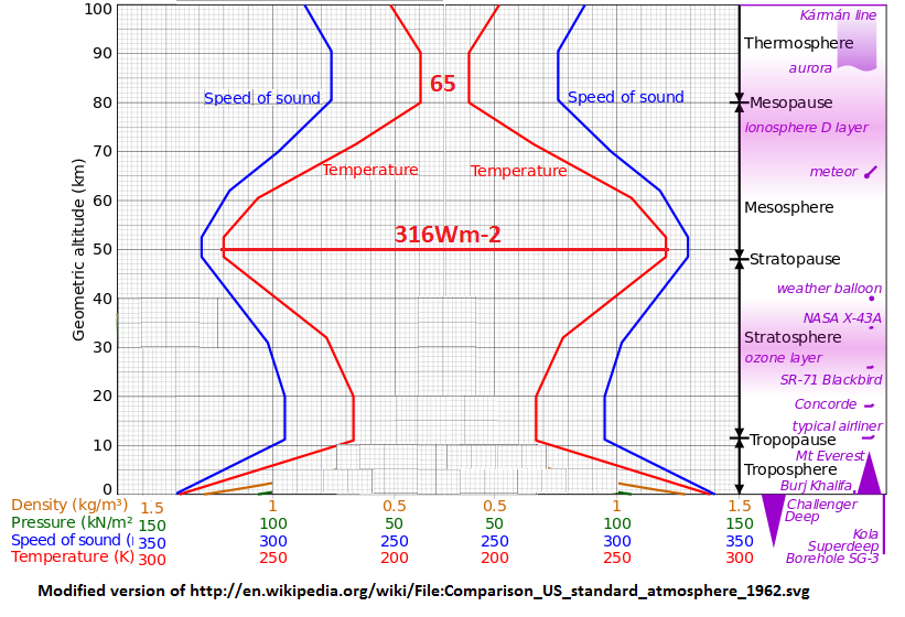
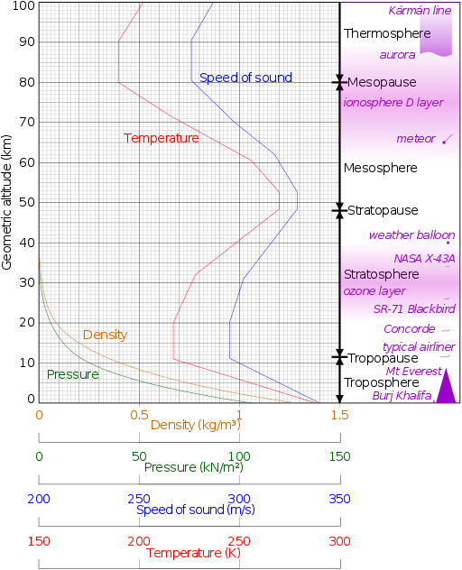
I used a spread sheet to show the basic relationships.  For the left hand Aqua world, Ocean efficiency increases while Turbopause efficiency increases.  The only limit is the 50% work done.  At 303.5 K degrees, [1-Tc(oceans)/Th] + [1-Tc(turbo)] = 0.5 or 50% of the available energy.  Remember that this is based solely on the two sink temperatures selected and the 50% requirement.  The effective energy of a surface at 303.5 K degrees is 481 Wm-2 which would require half of the energy available meaning the energy available is 962 Wm-2 or 70.7% of the solar constant of 1361 Wm-2.  Based on the simple Carnot Divider, the albedo or amount of energy reflected, should be 29.9% or the total energy available and just for fun, 29.9% of the available energy is 407 Wm-2.  The Tc(turbo) is based on a best guess, not a boundary based on sound physics.

Tc(turbo) if you follow my ramblings, is equal to the lowest temperature ever measured at the surface of the Earth.  A radiant reference "shell" should be perfectly isothermal.  Any temperature below -89.2 would not encompass the total surface area of Earth.  Tc(turbo) should be the first near ideal reference "shell" which also happens to be the approximate temperature of the Turbopause, where all turbulent mixing stops in the atmosphere approximately 100 kilometers above sea level.  This reference shell is obscured by the stratosphere temperature inversion, but so far the Carnot Divider appears to agree with my choice of atmospheric sink temperature.

The right hand "Real World" uses the Carnot divider to estimate land surface temperature assuming the oceans provide a portion of the energy to the land mass.   In this case the Carnot divider is a true divider.  From Land Tc(turbo) efficiency increases with surface temperature while the efficiency of heat transfer from the oceans decreases with land surface temperature.  At 50% combined efficiency, the land surface energy loss should be proportional to the total system loss.  This indicates a land surface temperature of 285.6K (12.45 C) would be ideal.  The "Ocean in" value is calculated using the Carnot Efficiency using the SST max to Land sink temperature with the ratio of ocean to land using the values at the top of the spread sheet.  The 12.45 C is slightly higher than the best estimate of actual land surface temperature and the 14.225 C is lower than the best estimate of the actual ocean surface temperature, but considering the small number of assumptions made, the estimates are pretty impressive. Most importantly the 33C and Albedo assumptions where not used and the albedo was actually discovered, indicating that the guess of Tc(turbo) was a good one.

There are a few things that need to be considered with this simple model.  The oceans system is enclosed in the atmospheric or Turbopause system.  The efficiency of the oceans system is 0.1063 or 10.63% of the 481Wm-2 input energy which would be 51.1 Wm-2 converted into thermal energy in the oceans.  That combined with the atmospheric work, 0.3937*481=189.4 equal 240.4 Wm-2 or the common value of the black body temperature of Earth which does not include the Turbopause shell effective energy of 65 Wm-2.

Since the Carnot Divider is based solely on temperatures, the 240.4 apparent black body energy plus the 65 Wm-2 Turbopause shell energy equal 305.4Wm-2 which would be a surface at a temperature at -2.24 C which is slightly lower than the -1.9 C Tc(oceans) value.  That would indicate that some minor tweaking of the sink temperatures is in order to close the energy balance, but for a simple dumb model, I would think it is worth a little more investment in time.

Another thing for some of the Sky Dragon Slayers to consider is that the Turbopause "shell" temperature is dependent on the radiant properties of atmospheric gases, primarily CO2.  This higher, colder "shell" or effective radiant layer is higher and colder than mentioned by the Climate Science Gurus, but is a purely radiant boundary. 

Finally for this post, the albedo energy of 407Wm-2 plus the Turbopause shell radiant energy of 65 Wm-2 is equal to 472Wm-2.  With 481 Wm-2 of work done in the systems via thermal energy, some portion of the 481-472=9 Wm-2 difference is likely due to non radiant energy input into the systems.  That would be gravitational, rotational and geothermal energy which combined may be on the same order of magnitude as CO2 forcing is estimated.

 Mo Carnot Stuff:

The Carnot Divider which uses one common source temperature with sink temperatures for two nested systems, produces what would be an ideal ratio of coupled system performance.  For the Aqua World example, ocean heat transfer efficiency plus atmospheric heat transfer efficiency or Energy in (Ein) has to equal the combined system inefficiency energy out (Eout).  If the sink temperatures are fixed, there is only one internal source temperature that will produce a "balanced" combined system. For a -1.9C ocean sink, Tc(oceans) and a -89.2 Atmosphere sink, Tc(Turbopause) the maximum common source temperature (Th) would be 30.35 C degrees. 

If Th increases, the atmosphere would warm more quickly than the oceans because of the different internal system efficiencies, producing an internal imbalance.  Since the ocean sink temperature is greater than the atmospheric sink temperature, where that imbalance exists and what would happen with an imbalance is not obvious.  So let's consider the third wiper on the Carnot Divider Diagram.  With Tc(oceans) = 271.25K and Tc(turbo) = 184K, the ocean sink to atmosphere sink efficiency is 1-184/271.25 = 0.322 or 32.2 % maximum efficiency.  The Carnot efficiency calculation is for a maximum efficiency, not an actual efficiency.  In a balanced system, the maximum heat transfer efficiency is 32.2 percent and with the source in this case being 271.25K degrees (307Wm-2), and the sink being 184K (65Wm-2), the total energy transfer would be 242 Wm-2 of which 32.2 percent would be 77Wm-2.  The actual sink temperature is 184K (65Wm-2) which if the transfer were ideal would be 77Wm-2 or 192.5K degrees. There is possibly 12 Wm-2 less energy transferred than could be transferred.  

There is more information in the ocean/atmosphere efficiency ratio.  At the 50% Ein=Eout requirement the Ocean efficiency from 303.5K to the 271.25K sink is 10.63% and the 303.5K source to 184K sink is 39.37 percent.  That ratio, 10.63/39.37=0.27, we can call the heat uptake ratio, which should be related to the specific heat capacities of the liquid (oceans) and gas (atmosphere) systems.  The specific heat of dry air is approximately 1.06 Joules per gram K at sea level and 273.15 K degrees and the specific heat capacity of salt water at 273.15K degree is 3.98 Joules per gram K at 273.16K degrees which would be a ratio of 26.6 percent. 

The Carnot Divider does not provide much information on the various internal states the system may take or the settling time between states, but is does indicate that there is a fairly narrow stable range dependent on maximum temperatures, not averages, and that specific heat capacity is a major consideration in the range of thermal efficiencies.

Mo Carnot Update:

		Aqua World Salt					Aqua World Fresh
	Ocean Sink	Turbo Sink	Ocean Max	Ocean Ave.		Ocean Sink	Turbo Sink	Ocean Max	Ocean Ave.
C degrees	-2.0000	-89.1500	30.2500	14.1250	C degrees	0.0000	-89.1500	31.5500	15.7750
K Degrees	271.1500	184.0000	303.4000	287.275	K Degrees	273.1500	184.0000	304.7000	288.925
Wm-2 (eff)	306.4937	64.9912	480.4469	386.1663	Wm-2 (eff)	315.6370	64.9912	488.7344	395.1150
Work	51.0692532146	189.0750025992			Work	50.6057406151	193.6010425433
Percentage		%Ocean		%Turbo	Percentage		%Ocean		%Turbo
0.5		0.1062953197		0.3935398813	0.5		0.10354447		0.3961273384
Combined		Tc(ocean)		Tc(Turbo)	Combined		Tc(ocean)		Tc(Turbo)
303.4		271.15		184	304.7		273.15		184

It looks like I got the size wrong, but this compares the Aqua World in salt and fresh versions.  If the Turbopause sink is fixed, then there would be a different control range for a salt and fresh ocean world.  The ideal maximum SST for Salt Aqua World would be 303.4 K degrees (note I added one significant digit) and the Fresh Aqua World would have an ideal maximum SST of 304.7 K degrees.  A 1.9 K degree change in the ocean sink would produce a 1.3K change in the maximum SST.   Fresh water flooding is often mentioned as a cause of THC stalling, but according to the simple Carnot Divider, the change in the freezing point would have a similar impact without all the complex modeling requirements.


I hope some of you could follow how effective even the simplest of models can be.  When a Carnot efficiency model can get this close it says something about the simplicity of the Earth Climate System once you eliminate the noise.

Note: I may come back to proof this later since this is a work in progress, so watch out for typos and mistakes.

I am finished with this one.  Now that I have double checked the "Real World" side of the first spread sheet I think there can be some improvements, but those will require actual area and shape considerations, for a simple model though, it is pretty amazing. 

SteveF, Webster and Greg Goodman Showcase the Confusion

I love how climate change discussion progress.  Over at Lucia's SteveF posted basically a rebuttal to the Foster and Ramsdorf much less than ideal removal of Solar, Volcanic and ENSO forcings to produce a theoretical CO2/Anthropogenic warming trend in the instrumental data.  SteveF's methods, also less than ideal but an improvement, indicates that there is a lower warming trend due to CO2/Anthropogenic forcings than the F&R method.  In the course of discussion, SteveF mentions that ENSO has no significant effect on "Global" temperature.

Greg Goodman enters promoting a dT/dt derivative approach which he thinks is the cat's ass of time series analysis methods which inspires Webster to throw in is fat tail opinion on the simplistic elegance of diffusion models and how CO2 follows the Indo-Pacific Warm Pool temperatures to near perfection. 

The elephant in the room is natural variability i.e. ocean pseudo oscillations, pseudo since couple oscillators respond differently to different perturbations and have differing dampening coefficients more often than not, with a range of potential time scales or Tau.  One can dig out "A" Tau, but in a chaotic coupled system, which is slightly redundant, never know for sure if that is "the" Tau relevant to the overall response.  In other words, the system is complex as all get out.

When Webster says that the IPWP and CO2 are joined at the hip, he is acknowledging that ENSO has a major impact on "Global" surface temperature and vice versa.  The based on his rather short time frame "Tau" decides that there is about 4 or so ppmv CO2 change per "Global" degree C change.  That is Ambrosia, the queen of fruit salads.

The Western Pacific is pretty close to Webster's Indo-Pacific Warm Pool and the hot end of the ENSO pseudo oscillation.  The Galapagos is near the original ENSO region which keeps moving to the west because we live on a planet that rotates once a day.  The CO2 is the first 22 thousand years of the Antarctic composite.  Until about 5 to 7 thousand years ago, CO2 and the ENSO regions where playing nicely just like Webster thinks.  But the oceans are never in "equilibrium".  There are 4300, 5000 and 5800 year orbital "cycles", sub-harmonics of the ~21ka precessional and ~41 ka obliquity orbital "cycles" with dampening rates that produce 1700, 1200, 1000, 400 etc. recurrent decay patterns in the paleo data.  The "average" lag of deep ocean temperature to surface temperature is around 1700 years, so every two to three "lag" periods can have a recurrent synchronized pulse that seems to come out of no where.  Which with the ocean distribution being asymmetrical, there is a bit of a hemispherical "seesaw" that likely never ends, just varies in amplitude like most couple oscillators are prone to do.  You can spend you whole life trying to figure those out or if you are lazy like me, note that +/-1 to +/- 2 C is a normal variance and don't worry about it, Tom Sawyer the hard stuff on some body else.

Now the interesting part of the discussion is that people are starting to notice that the "parsimonious" reasoning needs a bit of tweaking.  40 ppmv per degree C over longer time frames is an order of magnitude greater than the Webster's estimate.  This could get interesting.

Carnot Efficiency, OHC and Commander Kevin's Delima

The inspiration for this trash blog, as in a place to toss around ideas of my own that wouldn't vanish with a hard disk crash, was Commander Kevin's Earth Energy Budget.  Commander Kevin's budget did not balance and I caught quite a bit of grief from Commander Kevin's Space Cadets that seem to believe their fearless leader is infallible or some such nonsense.  Before Greame Stephens and other basically forced the Commander to admit his errors in the form of a "minor adjustment" in his latest version, others and myself have moved beyond the fatally flawed K&T/T&K/FTK etc. cartoons.

The loyal minions of the Commander though like dwelling in the past and have rejoiced that the Commander with another letter have reanalyzed the Ocean Heat Content data i.e. have beat the data to near submission, to show that the travesty has been averted, the prodigal heat returned.

I have used static models and Carnot efficiency estimates on a number of occasions to determine how much "slop" there is in the system.  That "slop" is the irreducible imprecision or the "you can't get there from here" uncertainty limits.  There is more "slop" aka natural variability, instrumentation error and the like, than there is CO2 forcing impact. 

Using Carnot efficiency and three points, yes three since there are liquid and gas "greenhouses", you can get a fair ballpark of what should be going on.

The Carnot efficiency as I have explained before is the "Maximum" efficiency possible with a hot reservoir and a cold reservoir.  Using absolute temperature, Ceff =1-Tc/Th, pretty simple fundamental Thermo 101 stuff.

Since salt water at about 35g/kg, or average ocean salinity, freezes at ~-2 C degrees (271.15K), we have one reliable reference.  As I have pointed out before the approximate temperature of the Turbopause is 184K, which happens to be the coldest temperature ever recorded on Earth's surface and also happens to be the approximate black body temperature of Venus, appears to be a pretty solid choice as the second cold reservoir.  The ocean surface temperature varies, but the maximum SST is close to 303K or 30C degrees.  But the SST maximum temperature varies. 

Using the two cold or Tc references for the liquid and gas parts of the problem with the ocean surface as a third reference, this chart slides SST maximum producing the range of efficiencies.  The red line at 50% represents the requirement for Ein=Eout.  Since each of the efficiencies represent work potential, when the total work done is equal to the waste energy, we would have a stable open system.  That stable maximum SST would be ~303K or about 30 C degrees, just like it is in nature.

At that point, the work done on the ocean is about 10% of the potential work that could be done.  Ten percent of the energy difference between the 30C surface and the -2C ice point is ~18Wm-2 ( that is the work done as energy flux) and 39 percent of the 30C to 184K Turbopause reference is ~160 Wm-2.  The energy converted to work is 178Wm-2 which would equal the energy lost or 356Wm-2 total energy was involved which, since we are using Wm-2, should be the average energy of the surface provided the area of the oceans is equal to the area of the Turbopause.  The areas are not equal.  The area of the Turbopause "shell" is about three percent larger than the true surface area of the Earth and the area of the oceans is only about 70% of the true surface area of the Earth.  Assuming 356Wm-2 is relevant only to the oceans area, then the "average" energy out would be ~241 Wm-2 for a surface the area of the true Earth surface.  That is a maximum.

For "normal" operation, the work done on the oceans would be 10% or less because the system is limited by the Ein=Eout requirements.  Normal is in quotes because poo-poo occurs.  Recovering from some event, the "average" energy of the oceans could be reduced meaning the system is not in a steady state but a start up mode where less energy could be converted to work in EITHER system, liquid or gas.  The systems are coupled by the common source or Th, so there can be damped oscillations as the systems approach individual and coupled steady states. 

I hope that is not too confusing, but if Commander Kevin had realistic understanding of even the simplest of coupled open systems, his minions might not be so befuddled. 

Back to the Layered Cocktail Analogy

You have three blocks with thermal mass.  The center block has a value of 400 units while the upper a lower blocks are fixed at 300 units.  There is a net heat flux of 100 units up and down.  Just like pouring a fancy layered cocktail, you slide a different density layer in between the lower two blocks.  What happens to the net energy flux? 

If the layer slide in is warmer than 300 units but colder than 400 units, there is less net flux down from the 400 block, but about the same net flux into the lower block.  The 400 block can cool more efficiently upwards.  The total energy of the "system" increases by whatever energy is transferred in by the slide layer.  If the slide layer has lower thermal mass, it would quickly "temper" to the average energy of the upper and lower blocks.  If the slide layer has high thermal mass, "tempering" will take longer and if the layer is an actual flow, heat will be transported elsewhere. 

This squiggly mess is the UAH lower stratosphere NH data, inverted and normalized with the deep ocean temperatures also normalized.  Believe it or not, there is actual useful information in that mess.  The two arrows show a lag between the deeper ocean and surface mixing layer (0-100 meters) at the 1998 super El Nino event.  The deep ocean data is annual while the NH LS is monthly with 25 month smoothing.  While there is a lot of other noise, the NH LS makes a pretty good proxy for volcanic forcing.  With the NH LS inverted, the relationship between ocean heat capacity is a little more obvious.  The lower stratosphere tends to track the average energy of the deep oceans 0-700 and 0-2000 meters than it does the surface mixing layer which can have a more complex lead/lag relationship with the deep oceans and volcanic forcing.  The lead/lags and short term divergences are mixing "noise" as various layers attempt to regain a steady state.  Since the deeper oceans are not cooled from above, the layered cocktail analogy applies.  Cooler more dense surface waters from the polar regions "slide" into place based on their temperature and density.  Trying to figure out the short term impact is not something I would dedicate my life to, but having a rough idea of the lag times is nice.

When you have a number of references that tend to be related to the delta Q part of the simplistic "Climate Sensitivity" equation, even this squiggly mess is useful. 

Deep Ocean Temperature versus the Surface

Because of the travesty of the missing heat the miraculous layer jumping 10 raised to the 22nd Joules of energy times some number depending on you choice of baseline is again the topic of climate geek conversation.  Using the standard normalizing data torture, this chart compares the Hadley Center SST3v data with the "global" deep ocean temperature.  No muss, no fuss, no scaling required, just divide by the standard deviation for a common period, in this case, 1955.5 to 2012.5 'cause that's how the deep ocean temperature was formated.  Nit pickers will say that the OHC data sucks.  Well, it doesn't suck much worse than any of the other data.  The absolute values they stick to the anomalies may suck, but the anomaly data does capture the general trends.  There is a little lead lag situation which I would think one should expect with an inconsistent relationship depending on who is leading, but the data should be quite "usable".

There does not appear to be any wild revelations of causations, just the typical complex mixing of the oceans that no one can come close to properly modeling.  The temperature trend difference between the 0-700 meter and 0-2000 meter data is barely noticeable to the point of likely not be significant, so harping on the small deviation at the end following a shift in instrumentation is a bit silly, but whatever floats your boat.

For Lucia's Crew - What is a Black Body Cavity?

A black body cavity is any energy source where the temperature of that source can be accurately approximated with the Stefan-Boltzmann Law.  That definition varies a bit from others, but it is the bottom line.  If the black body source is less than ideal, then you have to consider individual elements and their radiant spectra to adjust for the less than ideal source.  Depending on the level of precision that your application demands, you can assume "ideal" behavior as long as you remember the degree of uncertainty.

Pretty simple for most radiant physics/climate science geeks, there is uncertainty that needs to be considered whenever assuming ideal conditions.  ASSUME is the first real law of thermodynamics.

If you consider what makes a good black body cavity, the first thing would be consistency or stability.  The black body cavity is a reference, if your reference is noisy the adjustments for "less than ideal" behavior become more complex.  If you want to simplify the problem you pick a stable FRAME OF REFERENCE (FOR).  FOR is the second real law of thermodynamics.

By selecting a stable FOR and avoiding ASSUMEd precision that may not exist, you are following the first and most important real law of thermodynamics, KEEP IT SIMPLE STUPID, KISS.

SteveF at Lucia's has a post on removing natural variability from the global surface temperature record to show that another attempt to remove natural variability from the global surface temperature record was flawed and that the actual "trend" in actual global surface temperature is a gnat's ass less that estimated in the flawed attempt to remove the gnat's ass.  The author of the original gnat's ass paper snidely points out that SteveF's paper has residual gnat's asses circa 1976 which totally invalidates SteveF's gnat's ass removal procedure.

Welcome to climate science, home of fat tails, gnat's asses and elephant avoidance.

The elephant is still the black body cavity that provides the energy which everything else responds to.  Instead of a slit in a furnace or high precision optical source we have about 362 million kilometers squared of slit which can have non-uniformly distribute sea ice that can vary the slit area by 20 to 50 million kilometers squared or about 5.5% to 13.8% roughly on times scales of months to millions of years.  With all that range of possible variation, the temperature of the black body cavity, the global oceans, varies by about 3 degrees from a low of ~1 C to a high of ~4 C if you consider the "average" temperature of the black body cavity.  With the temperature of the black body cavity at the high end of the range, 4 C, which if it were an ideal black body cavity, would have an effective emissive energy of 334.5 Wm-2.  The Black body cavity is not ideal.  The temperature/effective energy varies from nearly 30 C at the equator to nearly -2 C at the poles for the surface or slit/aperture which is oddly the selected FOR for the gnat's ass assessors who ASSUME the energy is uniformly distributed and can only be significantly impacted by radiant forcing in a nearly linear manner.  Is that KISS?

The simple fact avoided is that the black body cavity cannot emit energy any more quickly than that energy can be internal transferred from the "average" of the black body cavity to the "slit", aperture, surface or radiant "shell", i.e. the ocean-atmosphere boundary layer.  How efficiently the black body cavity can transfer that energy internally determines the "average" energy of the black body source.

There can be several volumes published on the different factors that have different degrees of influence on the "average" temperature of the oceans aka black body source.   For now just consider that the oceans have an "average" temperature and that there is an "average" ice free ocean area.  With that average temperature equal to 4C (334.5Wm-2) and the average area equal to 360 kilometers square or 71 % of the total "surface" area of the globe, the "average" energy at any arbitrarily selected altitude would be equal to 334.5 Wm-2 times the ice free ocean area divided by the area of the arbitrarily selected "shell".  If we select a "shell" equal to that total sea level surface area of the Earth, then the effect radiant energy at that "shell" would be 334.5 time 0.71 equals 236 Wm-2, that is the FOR selected by climate science convention.  What about that other 29%?

During the black body mode or night mode, a large portion of that area is covered by ice and the remainer has a lower specific heat content relative to the black body source with much lower rates of internal heat transfer.  Where the "land" portion, as in not ice covered, has higher moisture content, that portion would have a significant impact on the "average" energy at the arbitrarily selected "shell", but energy from the true energy source would be transferred at differing degrees of efficiency to the "land" area.  By selecting the 236 Wm-2 altitude as a reference, the climate scientist now has to consider the ocean internal heat transfer efficiency and the ocean-atmosphere heat transfer efficiency and the ocean-"land" heat transfer efficiency.

Since the "land" is not symmetrically distributed, the ocean internal energy would not be uniformly distributed and with a rotating black body source, the hemispheres of the spherical source would be somewhat isolated by Coriolis effects.  Even with all this to consider, there is still an "average" energy of the oceans and an "average" energy of any arbitrarily selected radiant "shell".  By selecting a less arbitrary "shell", one that is more stable and uniformly distributed, like say the Turbopause, one could determine a range of natural variability, if either has a reasonably accurate long term estimated temperature/energy range.

Since both the energy and the ice free surface area varies over long times scales, the most stable FORs still do not eliminate uncertainty.  With a 1 C to 4 C "average" ocean temperature range, there would be an "average" 2.5 C (327.4 Wm-2) temperature/effective energy with a +/- 1.5 C (7.12Wm-2) range for the more recent glacial/interglacial periods.  If the focus is on either interglacial or glacial, the range could be reduced by half to +/-0.75 C (3.62 Wm-2).

So while I am just tickled to death that SteveF is winning the gnat's ass war, the real focus should be the expected range of natural variability on all relevant times scales, not just dreaming up more creative ways of removing a portion of the natural variability on arbitrary times scales, since the chart above doesn't paint the same pictures and these next two charts.

The more variably Northern Hemisphere versus the Indo-Pacific Warm Pool and

the rest of the world "surface" temperatures.  Which indicates a range in the ballpark of +/- 0.75 C (3.62Wm-2) uncertainty with time scales of at least 400 years.  Which by the way is roughly the time required for the "global" (0-2000 meters) ocean average temperature to rise, 0.75 C degrees. 

As a final note, while there are plenty of theories, part of the equation is sea ice area and hemispherical distribution.  The solar-lunar connection with climate likely plays a role in this variability since sea ice floats and orbital forcing also effect tides which can free or fix sea ice.  That is a non-radiant "forcing" or "unforced variable" in the currently radiant centric gnat's ass modeling approach. 

Deep Oceans Versus Surface Temperature

With the rate of warming slowing the big numbers in Ocean Heat Content (OHC) pops up as a diversion. Those big numbers, Joules times 10^22 are based on temperature change from an estimated "normal" total OHC.  The data for the OHC estimates is spotty at best even with the ARGO float system that started in 2002.  The depth of the OHC estimate is now down to 2000 meters or about half of the ocean volume.  On the bright side, since deep ocean temperatures are so stable, the confidence intervals are very small because nothing much changes, temperature wise.  Capacity wise, the numbers are big because the mass of the oceans is in the ballpark of 1.4 time 10^21 kilograms.  With everything based on surface temperatures and energy flux, throwing Joules time 10^22 in to the mix can get confusing.

Luckily, NOAA also has the deep ocean data in plain old temperature. 

The average temperature of the global oceans down to 2000 meters has changed about 0.08 C since 1955.  About 0.6 C of that has been since 1980 which is the baseline of choice for the ocean data guys.  I am not a big fan of the whole "global" thing or arbitrary baselines.  I am a fan of very stable frames of reference though.

This chart has the hemisphere deep ocean temperature anomaly compared to the Hadley version 3 sea surface temperature.  They are adjusted to a common 1955 to 2012 baseline and I have added a scaling factor of 5 for the large differences in the anomalies.  That is just eyeball scaling so don't try to get to crazy with make more of the chart than is there.

As I have mentioned before volcanic forcing impacts the NH more strongly than the SH.  The NH ocean heat capacity is discharged more quickly, not hard since the average NH SST is 3 C greater than the SH, and the SH thanks to the Antarctic Circumpolar Current just keeps transferring energy north until things get rebalanced.  Once the NH recovers from the volcanic cooling, then the oceans can start either warming in unison or do the seesaw thing.  The temperature change for the deep oceans during all this is pretty small and takes a long time.  Six hundreths of a degree per 33 years, if that is an "average" rate of gain, would be 0.18 C per century or about 444 years per every 0.8C of deep ocean warming.  That would mean it would take about 1700 years for a 3.06 C increase in deep ocean temperature at that rate of gain.

As I said, the "average" is kind of important since the oceans tend to like the 4 C average temperature with the ACC on the job keeping the NH about 3 C warmer than the SH.  Since the NH and SH can have nearly equal temperatures with the same 4 C deep ocean you could have a +/- 1.5 C swing around whatever that "average" temperature might be.  How that +/- 1.5 C change in "average" SST translates to the "average" surface temperature could be anyone's guess, but since most of the ice sheets are gone, it is pretty unlikely that there is a great deal more warming in the "pipeline". 

Since the deep ocean temperature scales pretty well with the surface temperature, I will leave with this little chart of past Indo-Pacific Warm Pool SST using the Oppo 2009 data.

It still looks to me like "most" of the warming is not due to CO2 unless CO2 depletion caused the last Little Ice Age. 

On Ocean Heat Transport - the Stumbling Block

Increased ocean heat transports and warmer climate

1. D. Rind
2. M. Chandler  DOI: 10.1029/91JD00009

We investigated the effect of increased ocean heat transports on climate in the Goddard Institute for Space Studies (GISS) general circulation model (GCM). The increases used were sufficient to melt all sea ice at high latitudes, and amounted to 15% on the global average. The resulting global climate is 2°C warmer, with temperature increases of some 20°C at high latitudes, and 1°C near the equator. The warming is driven by the decreased sea ice/planetary albedo, a feedback which would appear to be instrumental for producing extreme high-latitude amplification of temperature changes. Resulting hydrologic and wind stress changes suggest that qualitatively, for both the wind-driven and thermohaline circulation, the increased transports might be self-sustaining. As such, they would represent a possible mechanism to help account for the high-latitude warmth of climates in the Mesozoic and Tertiary, and decadal-scale climate fluctuations during the Holocene, as well as a powerful feedback to amplify other climate forcings. It is estimated that ocean transport increases of 50–70% would have been necessary to reproduce the warmth of various Mesozoic (65–230 m.y. ago) climates without changes in atmospheric composition, while the 15% increase used in these experiments would have been sufficient to reproduce the general climatic conditions of the Eocene (40–55 Ma). A companion experiment indicates that increased topography during the Cenozoic (0–65 Ma) might have altered the surface wind stress in a manner that led to reduced heat transports; this effect would then need to be considered in understanding the beginning of ice ages. Colder climates, or rapid climate perturbations, might have been generated with the aid of such altered ocean transports. The large high-latitude amplification associated with ocean heat transport and sea ice changes differs significantly from that forecast for increased trace gases, for which water vapor increase is the primary feedback mechanism. The different signatures might allow for discrimination of these different forcings; e.g., the warming of the 1930s looks more like the altered ocean heat transport signal, while the warming of the 1980s is more like the trace gas effect. The actual change of ocean heat transport and deep water circulation both in the past and in the future represents a great uncertainty.

For some reason there is still an issue with the relative importance of meridional and zonal energy flux control primarily by ocean pseudo-oscillations.  The last part of this abstract has the required "is more like a trace gas effect" which is one of those funding security blurbs.  The trace gases likely have an impact but change in ocean heat capacity would have the same "look".

 I put together this chart with the GISS and Hadley Center surface station data using their monthly versions by hemisphere.  Hadley also has a tropical of 30-30 global surface temperature anomaly.  The start data 1915, was selected because it was the lowest common point of all of the data sets making it more likely to be a truly "global" event.  The noisiest data set, GISS NH was used to determine the 2 sigma or 95 percent confidence range around the mean and the linear regression extended to 2060 where the GISS loti data set regression intersects the upper 2 sigma boundary.  Be my guest, pick out the trace gas "signature".

Since the ENSO region is used as a climate variable, I found a paleo reconstruction of the Indo-Pacific Warm Pool by Oppo that shows that pre-1915, the IPWP was warming from a two sigma event circa 1700 AD.

This is the Oppo IPWP reconstruction with the ever popular Central England temperature record.  Not a perfect match but a pretty fair correlation.

Here is the full Oppo reconstruction with the Hadley Center 30-30 (tropics) splice to the end with some massaging to get the decadal "bins" centered.  That is an excellent fit.  Where do you imagine the +/- 2 sigma range would be on this chart?  That's right, the "hemisphere" monthly noise range is about equal to the normal range of natural variability at least since 0 AD.  The hemispheres are seasonally 180 degrees out of phase in the mid to upper latitudes so a change in the seasonal heat distribution produces about the same "global" surface temperature impact as a longer term ocean pseudo-oscillation would produce.  If you have enough time, these pseudo-oscillation will average to some zero impact, how long do you have to wait?

Based on the Oppo reconstruction, about 1000 years.  I can confidently say that today is warmer than it has been in about 800 years, but 900 years ago it was likely warmer.  Since the warmer and cooler never got outside the 2 sigma range, about the best accuracy you can expect with paleo reconstructions, I could also say there has been no significant change in "Global" surface temperature for the past 2000 years. 

If you are a fan of BEST land only data to make your point, since it has a larger variance or standard deviation, the 2 sigma range would be larger.  We could probably take insignificant back to the Roman optimum or the very beginning of the Holocene.

"Global" climate doesn't change much, but regional can have 20 degree swings, possibly more.  We need to get past this ocean heat transport stumbling block and cut out the statistical games if climate science is going to more forward.

Just my two sigma cents.

Slushball Earth Entropy Budget ala Nick Stokes

Nick's Entropy Balance starts with the snowball Earth aka Weak Young Sun Paradox.  Earth has a weak sun or no GHG atmosphere with 30% albedo.  In his figure one above the "Ground" equilibrium is 922 Wm-2 in Nick's heat/entropy flux convention.  The red arrow represents heat flux, the head of the arrow is entropy transferred to the heat sink and the tail of the arrow entropy associated with the source of the flux.  For the incoming arrow, 102 Wm-2 is reflected and 235 Wm-2 thermalized corresponding to the common assumption of 30 percent albedo and 70% absorption producing "real" heat energy, the 235 and real energy reflected, the 102.  The 922 Wm-2 is unrealized energy basically.  With the Ground perspective or frame of reference the 922 Wm-2 entropy transferred to the heat sink is not utilized or thermalized, within the boundaries of the model. 

This is a large amount of energy partially because the thermalized energy is part of a spherical shape reduced to a simple up/down "average" and partially because of the radiant balance "convention".  If all of that entropy were themalized in this perspective, then thermal energy up would be 922/2 or 461 Wm-2 with a counter balancing 461 Wm-2 down, producing a radiant "shell".  Then if the energy were adjusted for the spherical shape, 461/4=115.6Wm-2.  This represents a small error in Nick's model, in my opinion, as the entropy should balance the "shell", in this case Ground thermalized energy for whatever common shape the shell takes. 

The reason is that the entropy can be thermalized and then released again as entropy from a secondary process, internal energy transfer for example, which can be any combination of mechanical, chemical or electromagnetic energy flux progressing over any time frame.

By adding the sub-surface to the diagram, you have the basic Slushball Earth which because of the thermal properties of the subsurface, mainly salt water, the minimum energy range for liquid water is dependent on the salinity of the fluid.  Assuming that the minimum temperature of a liquid sub-surface is 4C and the area of that sub surface is 70% of the total area of the sphere, the value of the sub-surface adjusted for area and shape would be 234.2 Wm-2.  The "Ground" in the slushball Earth case has a gap creating the equivalent of a Black body Cavity.  In the real world, the Ground surface would never be exactly 255K, but would have a range that changes with the seasons, centuries and millennia and a subsurface that would have an equal value that is rock solid stable by comparison, having had eons to approach a more realistic equilibrium. 

Again, Nick's post is here for reference.

Entropy Budget for Earth - Discussion of Nick Stokes Stab at it.

Since the typical climate blog fair lately really sucks, I was wandering around Nick Stokes' Moyhu blog when I came upon his stab at an Earth Entropy budget.  My static model approach doesn't try to pick out entropy or work since I think that is a couple of steps ahead of the current game.  The first hurdle is the Ground and Shell that Nick uses versus the black body cavity and shells that I use.  "Ground" or "surface" are too vague and subject to advection aka meridional and zonal heat flux which complicates modeling.

The red 40 in Nick's drawing is the problem.  I first started this blog because I discovered an 18 to 20 Wm-2 error in the K&T Earth Energy Budgets that produced the nearly double estimate of that "window" relative to that "Ground" surface.  If you are off by 18 to 20 Wm-2 because of poor choices of frames of reference, things will not get any better anytime soon.  When some of the top minds in the climate science game make such a mistake, getting them to admit it is rather difficult.

To show the problem instead of "Ground" I use the Black Body Cavity i.e. the global oceans which have a much more stable temperature.  The only problem with that frame of reference is that the oceans only cover ~70% of the "surface".    The big benefit though is that the reference has stayed within a degree or so for a very long time.

I added the Ocean BBC with shell on the side.  If the oceans covered 100% of the surface the shell would be 233K degrees based on half the energy of the source.  Since the oceans only cover 70% of the surface, the shell is appoximately 213.2 K with an approximately 20 Wm-2 "window" energy based on the Stephens et al. budget.  Since ~ 50 Wm-2 of the source energy is advected to produce a uniform shell, the actual "window" would more likely be 25 Wm-2 or half of the advected energy, which would be self absorbed during the advection.

Since the "shell" is simply a frame of reference, using the ocean 334.5 Energy and 70%, 234 Wm-2 could also be used producing the apparent ~236 Wm-2 average OLR value.  This simple approach does not include atmosphere SW absorption, but since the source 334.5 Wm-2 is a product of all radiant forcing over a large time scale, it is fairly easy to include a "surface" and atmospheric boundary layer to extend the budget.

With this modified Stephens et al. Budget cartoon, just adjust the 345.6 +/- 9 DWLR value to 334.5 +/- 9, where the +/- 9 is more likely plus and a good portion due to entropy produced by ocean and atmospheric circulation which has been estimated in the 4 Wm-2 range. 

You can visit Nick's blog post here but I need to look at what impact the revision of the "window" his estimates, but this 288K "Ground" legacy error appears to be gumming up the works.  Until the impact of that 20Wm-2 error is recognized with something more than a note saying that a "minor adjustment" was made to the budget, not much is going to happen.